![]()
LIBOR Market Model
Overview
The LIBOR Market Model (LMM) is an interest rate model
based on evolving LIBOR market forward rates.
It is also known as the Brace-Gatarek-Musiela (BGM) model, after the
authors of one of the first papers where it was introduced (Ref [2]). In contrast
to models that evolve the instantaneous short rate (Hull-White,
Black-Karasinski models) or instantaneous forward rates (Heath-Jarrow-Morton
model), which are not directly observable in the market, the objects modeled
using LMM are market-observable quantities (LIBOR forward rates). This makes LMM popular with market
practitioners. Another feature that
makes the LMM popular is that it is consistent with the market standard
approach for pricing caps using Black’s formula.
The LMM can be used to price any instrument whose pay-off
can be decomposed into a set of forward rates.
It assumes that the evolution of each forward rate is lognormal. Each forward rate has a time dependent volatility
and time dependent correlations with the other forward rates. After specifying these volatilities and
correlations, the forward rates can be evolved using
The standard lognormal LMM does not produce the
market-observed caplet volatility smile/skew (Ref [3]). To produce a
skew, the LMM can be extended to incorporate a local volatility model, a
stochastic volatility model, a jump diffusion model, or some combination of the
above. FINCAD provides pricing functions
that permit the use of three different versions of the LMM: (1) the standard
lognormal LMM, (2) the LMM enhanced with a Constant Elasticity of Variance
(CEV) local volatility process, and (3) the LMM enhanced with a Displaced
Diffusion (DD) local volatility process.
The next section discusses the standard lognormal LMM in detail. A sub-section at the end discusses the local
volatility extensions.
Formulas & Technical Details
Lognormal LIBOR Market Model
Assume that there are ![]() forward rates
forward rates ![]() that describe the
pay-off of an interest rate derivative.
The evolution of each forward rate
that describe the
pay-off of an interest rate derivative.
The evolution of each forward rate ![]() is described by
the stochastic differential equation:
is described by
the stochastic differential equation:
![]()
Equation 1
where
![]() is a standard Wiener
process and
is a standard Wiener
process and
![]() is the instantaneous
correlation between forward rates
is the instantaneous
correlation between forward rates ![]() and
and ![]() .
.
The instantaneous lognormal volatility and drift of
forward rate ![]() are
are ![]() and
and ![]() , respectively.
Note that the drift
, respectively.
Note that the drift ![]() for forward rate
for forward rate ![]() can be calculated
from the other forward rates and their instantaneous volatilities and
correlations (see Joshi for more details Ref [7]). Thus, the
instantaneous volatilities and correlations completely describe how forward
rates will evolve in the future. The
first thing to do is to specify the instantaneous volatilities and
correlations.
can be calculated
from the other forward rates and their instantaneous volatilities and
correlations (see Joshi for more details Ref [7]). Thus, the
instantaneous volatilities and correlations completely describe how forward
rates will evolve in the future. The
first thing to do is to specify the instantaneous volatilities and
correlations.
There are three main approaches for determining the
instantaneous volatilities and correlations of forward rates (Ref [12]):
1. They
can be obtained from analyzing historical data.
2. They
can be obtained by calibrating the model to current market prices of caplets
and European swaptions.
3. The
user can explicitly specify volatilities and correlations based on how he or
she believes they will evolve in the future.
A combination of these three approaches can also
be used.
Calibration
FINCAD provides functions for calibrating (see the Calibration FINCAD
Math Reference document) the instantaneous volatilities and correlations of the
LMM to quoted market data for caplets and European swaptions. The calibration of the LMM is a delicate
issue and is still an area of active research (Refs [3], [12], [13]). Calibrating
time-dependent instantaneous volatilities and correlations of a set of forward
rates to market data can be a difficult task.
To simplify the calibration procedure, the LMM calibration
functions use restricted functional forms (presented in recent literature Refs [3], [7], [6]) for the instantaneous volatilities and
correlations. The trade-off in using
restricted functional forms to make the calibration procedure easier is that
they may not be able to fit all market conditions. By calibrating using restricted functional
forms, the approach taken is really a combination of approaches 2 and 3 as
discussed in the previous section. This
is because choosing a functional form limits how forward rates can evolve in
the future. Even though calibration is
performed on market data, the choice of the functional form places restrictions
on how the rates can evolve.
The FINCAD LMM calibration functions use the following
functional form (or parameterization) for the instantaneous volatilities of
forward rates:
![]()
Equation 2
This linear-exponential parametric form is a
time-homogeneous form, which means that the instantaneous volatility of a forward
rate is not a function of the current date but only a function of the time
until the rate is set. The parameters ![]() allow for the
exact fitting of specific forward rate volatilities to quoted caplet volatilities.
This parametric form is able to produce both a monotonically decreasing and
“humped” structure of the instantaneous volatility, consistent with features
observed in the market. In addition, the parameters
allow for the
exact fitting of specific forward rate volatilities to quoted caplet volatilities.
This parametric form is able to produce both a monotonically decreasing and
“humped” structure of the instantaneous volatility, consistent with features
observed in the market. In addition, the parameters ![]() can be interpreted in
financial terms. For very long maturities i.e. when
can be interpreted in
financial terms. For very long maturities i.e. when ![]() is large, the
instantaneous volatility approaches
is large, the
instantaneous volatility approaches ![]() . Therefore we can interpret
. Therefore we can interpret ![]() as the
volatility of forward rates very far in the future. Generally, this parameter
should have a positive value. The parameter
as the
volatility of forward rates very far in the future. Generally, this parameter
should have a positive value. The parameter ![]() can be
interpreted as the rate at which the volatility approaches the limit
can be
interpreted as the rate at which the volatility approaches the limit ![]() . For forward rates with very short maturities, i.e.
when
. For forward rates with very short maturities, i.e.
when ![]() approaches zero, we
can see the instantaneous volatility approaches
approaches zero, we
can see the instantaneous volatility approaches ![]() . This leads us to conclude that this quantity should
also be greater than zero. We can gain some insight into the location of the
hump in the volatility structure by evaluating
. This leads us to conclude that this quantity should
also be greater than zero. We can gain some insight into the location of the
hump in the volatility structure by evaluating ![]() From this we find that the hump is located at
From this we find that the hump is located at ![]() Therefore, a hump will
only be present for
Therefore, a hump will
only be present for ![]() Under normal circumstances, we observe a volatility structure
similar to the one shown in the Figure 1 (using parameter values from Joshi [7] and Jaeckel [6]). The initial positive slope allows us to infer the
further restriction that
Under normal circumstances, we observe a volatility structure
similar to the one shown in the Figure 1 (using parameter values from Joshi [7] and Jaeckel [6]). The initial positive slope allows us to infer the
further restriction that ![]() in this case. For more
details see Brigo and Mercurio [3], Joshi [7] and Jaeckel [6].
in this case. For more
details see Brigo and Mercurio [3], Joshi [7] and Jaeckel [6].
Figure 1
The FINCAD LMM calibration functions use the
following functional form (or parameterization) for the instantaneous
correlations between forward rates:
![]()
Equation 3
This exponential parametric form is not time
dependent (i.e., it does not depend on the
current date nor the times until the two forward rates are set, but only on the
difference between the two times). It is
discussed by Molgedey [9]. It is also a
more general case of forms presented by Joshi [7] and Jaeckel [6]. The figure
below shows the instantaneous correlation for some parameter values used by
Joshi [7] and Jaeckel [6]. The general
interpretation of this structure is that forward rates with similar maturities
show a high degree of correlation, while those with very different maturities are
less correlated. We see that when ![]() , the correlation is 1 as required. The parameter
, the correlation is 1 as required. The parameter ![]() can be interpreted as
the limit of instantaneous correlation that is approached for rates far
separated in time, while the parameter
can be interpreted as
the limit of instantaneous correlation that is approached for rates far
separated in time, while the parameter ![]() describes how fast the
correlation decreases and approaches
describes how fast the
correlation decreases and approaches ![]() . In terms of an instantaneous correlation matrix, this
parametric form describes a matrix with ones along the diagonal and values
decreasing at a rate of
. In terms of an instantaneous correlation matrix, this
parametric form describes a matrix with ones along the diagonal and values
decreasing at a rate of ![]() as we move away from
the diagonal. The limit that the far off-diagonal elements approach is given by
as we move away from
the diagonal. The limit that the far off-diagonal elements approach is given by
![]() .
.
It should be noted that the above specification of the
instantaneous correlation between forward rates does not entirely describe the
“terminal correlation” between the rates. i.e. the non-instantaneous
correlation. The terminal correlation is determined by a combination of both
the instantaneous volatility and correlation structures. See Brigo and Mercurio
[3]
for more details.
Figure 2
The FINCAD LMM calibration functions allow:
·
a functional form for instantaneous volatilities
to be fitted to caplet data (caplet data contains no information about
correlations).
·
a functional form for instantaneous correlations
to be fitted to European swaption data given a specified form for instantaneous
volatilities (obtained from calibration to caplets).
·
functional forms for both instantaneous
volatilities and correlations to be fitted simultaneously to European swaption
data alone.
For example, the FINCAD calibration functions
allow a user to calibrate the instantaneous volatility and correlation
parameters by (1) calibrating the volatility parameters ![]() , and
, and ![]() to caplet data;
then (2) holding these parameters fixed while calibrating the instantaneous
correlation parameters
to caplet data;
then (2) holding these parameters fixed while calibrating the instantaneous
correlation parameters ![]() and
and ![]() to swaption data (see
the Calibration
FINCAD Math Reference document for more information).
to swaption data (see
the Calibration
FINCAD Math Reference document for more information).
The exact procedure by which caplets and swaptions are
used to calibrate the instantaneous volatilities and correlations depends on
the particular pricing application. For
example, one practitioner (Ref [6]) does not calibrate the instantaneous correlations at
all. Rather, the correlation parameters
are set to values based on historical data.
The volatility parameters ![]() ,
, ![]() are calibrated to
caplet data, then a forward rate-forward rate covariance matrix is constructed (see
Equation 4
below). This matrix is transformed into
a swap rate-swap rate covariance matrix, which is then calibrated to swaption
data. In this way one obtains a
“calibration to European swaption prices whilst retaining as much calibration
to the caplets as possible without violating the overall FRA/FRA correlation
structure too much, which is typically exactly what a practitioner wants for
the pricing of Bermuda swaptions” (Ref [6]). A similar
procedure using the FINCAD functions would be to (1) set the instantaneous
correlation parameters
are calibrated to
caplet data, then a forward rate-forward rate covariance matrix is constructed (see
Equation 4
below). This matrix is transformed into
a swap rate-swap rate covariance matrix, which is then calibrated to swaption
data. In this way one obtains a
“calibration to European swaption prices whilst retaining as much calibration
to the caplets as possible without violating the overall FRA/FRA correlation
structure too much, which is typically exactly what a practitioner wants for
the pricing of Bermuda swaptions” (Ref [6]). A similar
procedure using the FINCAD functions would be to (1) set the instantaneous
correlation parameters ![]() and
and ![]() to values suggested in
the literature (
to values suggested in
the literature (![]() , see Ref [6]); (2) use the FINCAD functions to calibrate the instantaneous
volatility parameters
, see Ref [6]); (2) use the FINCAD functions to calibrate the instantaneous
volatility parameters ![]() , and
, and ![]() ; to caplet data; then (3) use the FINCAD functions to calibrate
the instantaneous volatility and correlation parameters
; to caplet data; then (3) use the FINCAD functions to calibrate
the instantaneous volatility and correlation parameters ![]() ,
, ![]() , and
, and ![]() to swaption data, using
a narrow range of allowed values for each parameter centered on the values determined
in steps (1) and (2) (see the Calibration FINCAD Math Reference document for more information).
to swaption data, using
a narrow range of allowed values for each parameter centered on the values determined
in steps (1) and (2) (see the Calibration FINCAD Math Reference document for more information).
Calibrated values of the lognormal volatility and
correlation parameters typically lie in the ranges:
·
![]() : -1 to 1
: -1 to 1
·
![]() : 0 to 0.5
: 0 to 0.5
·
![]() : 0 to 5
: 0 to 5
·
![]() : 0 to 0.5
: 0 to 0.5
·
![]() : 0 to 1
: 0 to 1
·
![]() : 0 to 1
: 0 to 1
The performance of the calibration functions with
respect to determining volatility and correlation parameters depends on the
characteristics and quality of the caplet and swaption data. For example, calibration using illiquid or
inaccurate data (see Refs [3], [13]) may result in function failure or incorrect
parameter values. Also, because the
calibration functions use restricted parametric forms for instantaneous
volatilities and correlations, there will be cases when the functions fail even
when the market data is liquid and accurate.
In these cases, users will have to use a combination of the three
approaches (described at the end of the previous section) for determining
volatilities and correlations.
In order to make the calibration functions more efficient,
closed form approximations are used to price European swaptions that do not
require
Pricing
Evolving the Forward Rates using Monte Carlo
Simulation
After specifying which forward rates to evolve and their
instantaneous volatilities and correlations, by calibration or other means, a
In particular, an ![]() covariance matrix
covariance matrix ![]() is built for each
user-defined forward rate evolution period, where
is built for each
user-defined forward rate evolution period, where ![]() is the number of
forward rates. For example, given that
is the number of
forward rates. For example, given that ![]() is the forward
rate effective at
is the forward
rate effective at ![]() and terminating at
and terminating at
![]() , then for the time period
, then for the time period ![]() , where
, where ![]() , the elements of the
, the elements of the ![]() instantaneous
covariance matrix are:
instantaneous
covariance matrix are:
![]() .
.
Equation
4
The
covariance matrix ![]() contains all the
information needed to evolve the forward rates from time
contains all the
information needed to evolve the forward rates from time ![]() to
to ![]() and can be
calculated from the restricted functional forms for instantaneous volatilities
and correlations. In particular, the
parameterization of instantaneous correlation in Equation 3 is time-independent, which means that instantaneous
correlation can be taken out of the covariance integral in Equation 4. The resulting integral can
be evaluated analytically using the functional form for instantaneous
volatility from Equation
2 (see Jaeckel [6]).
and can be
calculated from the restricted functional forms for instantaneous volatilities
and correlations. In particular, the
parameterization of instantaneous correlation in Equation 3 is time-independent, which means that instantaneous
correlation can be taken out of the covariance integral in Equation 4. The resulting integral can
be evaluated analytically using the functional form for instantaneous
volatility from Equation
2 (see Jaeckel [6]).
If the pay-off of the
instrument depends on the value of the forward rates ![]() at one future time
at one future time
![]() , the forward rates only have to be evolved for a single
time step from the value date
, the forward rates only have to be evolved for a single
time step from the value date ![]() to
to ![]() . This requires
only a single
. This requires
only a single ![]() covariance matrix
for time period t0 to t1 to describe the evolution of forward rates. If the payoff of the instrument depends on
the forward rates observed at
covariance matrix
for time period t0 to t1 to describe the evolution of forward rates. If the payoff of the instrument depends on
the forward rates observed at ![]() dates
dates ![]() ,
, ![]() , …
, … ![]() , the forward rates need to be evolved for m time steps from
, the forward rates need to be evolved for m time steps from ![]() 0 to
0 to ![]() ,
, ![]() to
to ![]() , …
, … ![]() to
to ![]() . To specify the
evolution of forward rates requires
. To specify the
evolution of forward rates requires ![]() separate
covariance matrices, one for each time evolution period.
separate
covariance matrices, one for each time evolution period.
Given the matrix
elements ![]() for a particular
time evolution period,
for a particular
time evolution period, ![]() is decomposed into
a pseudo square root via the Cholesky method, or via spectral decomposition if
the Cholesky method fails for any reason:
is decomposed into
a pseudo square root via the Cholesky method, or via spectral decomposition if
the Cholesky method fails for any reason:
![]() .
.
Equation 5
Equation
1 is then written as (Ref [6]):
![]()
Equation 6
where the ![]() are
are ![]() independent Wiener
processes. If one wishes to employ
“factor reduction” and evolve the forward rates using
independent Wiener
processes. If one wishes to employ
“factor reduction” and evolve the forward rates using ![]() independent Wiener
processes (Ref [6]), then Equation
1 is re-written as:
independent Wiener
processes (Ref [6]), then Equation
1 is re-written as:
![]() .
.
Equation 7
The
variances of the forward rates, ![]() , (obtained from calibration or directly from the
market-quoted implied volatilities of caplets) are retained by setting (Ref [6]):
, (obtained from calibration or directly from the
market-quoted implied volatilities of caplets) are retained by setting (Ref [6]):
 .
.
Equation 8
The FINCAD
implementation of the LMM uses the zero coupon bond maturing at time ![]() (i.e., on the terminating date of the
(i.e., on the terminating date of the ![]() forward rate,
forward rate, ![]() ) as numeraire, so the drift of
) as numeraire, so the drift of ![]() at time
at time ![]() is given by (Refs [3], [6]):
is given by (Refs [3], [6]):
 .
.
Equation
9
![]() is the accrual
factor for the rate term defined by
is the accrual
factor for the rate term defined by ![]() .
.
Because the drifts given
by Equation
9 are state dependent and therefore indirectly
stochastic, Equation
1 must be solved using a numerical scheme. FINCAD implements a log-Euler discretization
of the forward rate process (Refs [3], [6]):
![]() .
.
Equation
10
![]() is the drift from Equation 9, predicted using Equation 4 for the period
is the drift from Equation 9, predicted using Equation 4 for the period ![]() , then corrected using the “predictor-corrector” method (Ref
[6]) to take into account the fact that the
, then corrected using the “predictor-corrector” method (Ref
[6]) to take into account the fact that the ![]() change during the
evolution period.
change during the
evolution period.
Forward rates in the
standard lognormal LMM are evolved over successive time periods in a Monte
Carlo simulation according to Equation
10, given the forward rate-forward rate covariance matrix
![]() for each time
period. By generating many such paths of
forward rates, the expectation of a particular forward rate on a particular
date in the chosen probability measure (i.e., the
for each time
period. By generating many such paths of
forward rates, the expectation of a particular forward rate on a particular
date in the chosen probability measure (i.e., the ![]() -forward measure or terminal measure), conditional on
today’s value of the forward rate, is the average simulated value over all
paths. On each path of forward rates,
the coupons and the price of the numeraire asset are calculated on coupon
payment dates. Today’s value of the
numeraire asset is also calculated for the path. The coupons are discounted through the
numeraire and summed to get the price of the instrument on the path. The fair value of the instrument is found by
averaging over all paths.
-forward measure or terminal measure), conditional on
today’s value of the forward rate, is the average simulated value over all
paths. On each path of forward rates,
the coupons and the price of the numeraire asset are calculated on coupon
payment dates. Today’s value of the
numeraire asset is also calculated for the path. The coupons are discounted through the
numeraire and summed to get the price of the instrument on the path. The fair value of the instrument is found by
averaging over all paths.
User Defined Covariance Matrices
An input to the FINCAD
interest rate derivative pricing functions that use the LMM is a sequence of
covariance matrices, one for each time evolution period of the instrument. Utility functions are provided to generate
these covariance matrices, given the parametric forms for instantaneous
volatilities and correlations described above.
Instead of using the
calibration and matrix generation functions, users can define their own
covariance matrices and input them directly into the pricing functions. The following example describes how this can
be done.
The example assumes
an instrument whose pay-off depends on 4 forward rates. The first forward rate ![]() is from
is from ![]() , the second forward rate
, the second forward rate ![]() is from
is from ![]() , the third forward rate
, the third forward rate ![]() is from
is from ![]() , the fourth forward
rate
, the fourth forward
rate ![]() is from
is from ![]() and the current
date corresponds to time
and the current
date corresponds to time ![]() . Also, suppose
this instrument has a Bermudan structure and its pay-off depends on the forward
rates observed at times
. Also, suppose
this instrument has a Bermudan structure and its pay-off depends on the forward
rates observed at times ![]() , and
, and ![]() . Running the
simulation requires evolving the forward rates from
. Running the
simulation requires evolving the forward rates from ![]() ,
, ![]() ,
, ![]() and
and ![]() . Thus, four
separate 4 by 4 covariance matrices are required to describe the evolution of
forward rates, one for each time step that needs to be evolved.
. Thus, four
separate 4 by 4 covariance matrices are required to describe the evolution of
forward rates, one for each time step that needs to be evolved.
Now, suppose the user
wants to explicitly specify the instantaneous volatilities and correlations as
piece-wise constant functions (i.e.,![]() and
and ![]() are constants during
each time step) with the following values:
are constants during
each time step) with the following values:
From t0
to t1,

From t1
to t2,

From t2
to t3,

From t3
to t4,

Notice that the data
has a certain structure. For each time
period ![]() and
and ![]() if
if ![]() . This is because
for
. This is because
for ![]() i forward
rate
i forward
rate ![]() has already
expired because it is already past its starting time
has already
expired because it is already past its starting time ![]() . Forward rates
that have already expired cannot be evolved so they do not have volatilities
and correlations. So for this example,
from
. Forward rates
that have already expired cannot be evolved so they do not have volatilities
and correlations. So for this example,
from ![]() , the forward rates
, the forward rates ![]() have to be evolved;
from
have to be evolved;
from ![]() , forward rates
, forward rates ![]() have to be evolved;
from
have to be evolved;
from ![]() , forward rates
, forward rates ![]() have to be evolved; and from
have to be evolved; and from ![]() , only
, only ![]() has to be evolved.
has to be evolved.
Also, notice that the
non-zero diagonals of the instantaneous correlation matrix are always one and
the matrix is symmetric. This is because the correlation between ![]() and
and ![]() is the same as
that between
is the same as
that between ![]() and
and ![]() . Another
restriction on the instantaneous correlation matrix is that is it positive
definite. For more on restrictions for
instantaneous volatilities and correlations, see Ref [3].
. Another
restriction on the instantaneous correlation matrix is that is it positive
definite. For more on restrictions for
instantaneous volatilities and correlations, see Ref [3].
Given values for the
instantaneous volatilities and correlations, Equation 4 is then used to generate the covariance matrices. Because the instantaneous volatilities and
correlations are piecewise-constant, the integral is easy to evaluate. For example, to calculate the entry ![]() suppose that
suppose that ![]() and
and ![]() (in years). From Equation 4,
(in years). From Equation 4, ![]() using the values of
using the values of ![]() between
between ![]() and
and ![]() . Thus,
. Thus, ![]() .
.
Early Exercise in Monte
Carlo Simulation
When there is only
one possible exercise date (European exercise),
The FINCAD LMM
implementation uses the Least Squares Monte Carlo (LSMC) algorithm proposed by
Longstaff and Schwartz [8] to price instruments with early exercise
features. The LSMC algorithm works
backwards from the last exercise date to previous exercise dates as follows:
1. Calculate
the exercise value on the exercise date for each path. For Bermudan swaptions, the exercise value is
simply the value of the underlying swap, which is easily calculated “off the
curve” (Ref [12]).
2.
If this is the last exercise date, set the
continuation value = discounted continuation value = 0 for each path and go to
Step 6.
3.
For each path, set the continuation value on the
exercise date equal to the discounted continuation value from the later
exercise date.
4.
Regress the continuation values from each path
in Step 3 against a linear combination of “basis functions” evaluated at
“regression variables”.
5.
Use the regression parameters, regression
variables, and basis functions from Step 4 to estimate the continuation value
on the exercise date for each path.
6.
For each path, if the exercise value >
continuation value, then set the exercise flag for this date = TRUE and set
continuation value = exercise value. Otherwise,
set the exercise flag = FALSE and set continuation value = discounted
continuation value.
7.
Move to the previous exercise date.
8.
Repeat steps 1-7 until there are no more
exercise dates.
The earliest
date on each path for which exercise flag = TRUE is the optimal exercise date
for that path.
The exercise
strategy found by the LSMC algorithm is typically a sub-optimal exercise
strategy (at best, the optimal exercise strategy), so the price of the option
given by the LSMC algorithm is a lower bound on the price.
The choice of
regression variables and choice of basis functions affect how closely the LSMC
algorithm approximates the optimal exercise strategy, and depend on the
specific instrument being priced (Refs [8], [12]). The FINCAD
pricing functions provide a choice between two sets of regression
variables: either the 0th and
1st moments of the interest rate curve (i.e.,
the level and slope of the interest rate curve, represented by a swap price per
unit notional and a forward rate) or the sums of the random factors used to
evolve each forward rate. A choice
between two different sets of basis functions is also provided: either 2nd-order polynomials or 2nd-order
Laguerre polynomials. The price of an
instrument, e.g., a Bermudan swaption, is not
expected to be particularly sensitive to the basis functions. Instead, one should focus on selecting
regression variables that are indicative of continuation values relative to
exercise values (Ref [12]). The sums of
random factors are general variables that can be used for any derivative. In the case of swaptions, the 0th
and 1st moments of the interest rate curve are expected to be the
best choice for regression variables.
For more details on the choice of regression variables and basis
functions for Bermudan swaptions see Pedersen [11] and Piterbarg [12].
The LSMC algorithm is
described further in the Bermudan and American Style
Basket Options FINCAD Math Reference document.
Local Volatility Extensions
FINCAD provides two
local volatility extensions to the LMM in order to model implied volatility
skew: Constant Elasticity of Variance
(CEV) and Displaced Diffusion (DD).
Constant Elasticity of Variance
In the LMM
with CEV, Equation
1 becomes (Refs [5], [10], [14]):
![]()
Equation
11
so that Equation 9 becomes (Refs [1], [5], [10]):
 .
.
Equation 12
and Equation 10 becomes (Refs [1], [5], [10]):

Equation
13
where ![]() is the CEV parameter,
constant for all forward rates. That is,
forward rates in the LMM+CEV are evolved over successive time periods in a
Monte Carlo simulation according to Equation 13, given
is the CEV parameter,
constant for all forward rates. That is,
forward rates in the LMM+CEV are evolved over successive time periods in a
Monte Carlo simulation according to Equation 13, given ![]() and the forward
rate-forward rate CEV covariance matrix for each time period. The parameterization of CEV instantaneous
volatility and correlation for calibration of the covariance matrix retain the
same forms as shown in Equation
2 and Equation
3, respectively.
The standard LMM is recovered from the LMM+CEV by simply setting
and the forward
rate-forward rate CEV covariance matrix for each time period. The parameterization of CEV instantaneous
volatility and correlation for calibration of the covariance matrix retain the
same forms as shown in Equation
2 and Equation
3, respectively.
The standard LMM is recovered from the LMM+CEV by simply setting ![]() .
.
Note that Equation 13 is the log-Euler discretization of Equation 11. In a process
such as CEV where forward rate = 0 is possible, it is typically better to use a
direct Euler discretization of the stochastic differential equation (Ref [1]). However, for
typical market conditions where forward rate = 0 is improbable, the log-Euler
discretization works well.
Closed-form
expressions for the prices of caplets and European swaptions are available (Refs
[1], [3], [5], [10]) for calibration of the LMM+CEV. Typical values of the calibrated model
parameters are ![]() ,
, ![]() ,
, ![]() , and
, and ![]() for a negative
skew (caplet implied volatility decreases with strike rate), or
for a negative
skew (caplet implied volatility decreases with strike rate), or ![]() ,
, ![]() ,
, ![]() , and
, and ![]() for a positive skew
(caplet implied volatility increases with strike rate). When calibrating the LMM+CEV, one must
usually input large uncertainties for the calibration instruments (caplets or
swaptions) that are far from the money (see the Calibration
FINCAD Math Reference document), because these instruments have near-zero vega
which means the same price is obtained for a large range of volatilities.
for a positive skew
(caplet implied volatility increases with strike rate). When calibrating the LMM+CEV, one must
usually input large uncertainties for the calibration instruments (caplets or
swaptions) that are far from the money (see the Calibration
FINCAD Math Reference document), because these instruments have near-zero vega
which means the same price is obtained for a large range of volatilities.
Displaced Diffusion
In the LMM with
DD, Equation
1 becomes (Refs [7], [10], [14]):
![]()
Equation
14
so that Equation 9 becomes (Refs [1], [7], [10]):
 .
.
Equation 15
and Equation 10 becomes (Refs [1], [3], [10], [14]):
![]()
Equation
16
where ![]() is the DD
parameter, constant for all forward rates.
That is, forward rates in the LMM+DD are evolved over successive time
periods in a Monte Carlo simulation according to Equation 16, given
is the DD
parameter, constant for all forward rates.
That is, forward rates in the LMM+DD are evolved over successive time
periods in a Monte Carlo simulation according to Equation 16, given ![]() and the forward
rate-forward rate DD covariance matrix for each time period. The parameterization of DD instantaneous
volatility and correlation for calibration of the covariance matrix retain the
same forms as shown in Equation
2 and Equation
3, respectively.
The standard LMM is recovered from the LMM+DD by simply setting
and the forward
rate-forward rate DD covariance matrix for each time period. The parameterization of DD instantaneous
volatility and correlation for calibration of the covariance matrix retain the
same forms as shown in Equation
2 and Equation
3, respectively.
The standard LMM is recovered from the LMM+DD by simply setting ![]() = 0.
= 0.
Closed-form
expressions for the prices of caplets and European swaptions are available (Refs
[3], [10]) for calibration of the LMM+DD. Typical values of the calibrated model
parameters are ![]() ,
, ![]() ,
, ![]() , and
, and ![]() for a negative
skew (caplet implied volatility decreases with strike rate), or
for a negative
skew (caplet implied volatility decreases with strike rate), or ![]() ,
, ![]() ,
, ![]() , and
, and ![]() for a positive
skew (caplet implied volatility increases with strike rate). When calibrating the LMM+DD, one must usually
input large uncertainties for the calibration instruments (caplets or
swaptions) that are far from the money (see the Calibration
FINCAD Math Reference document), because these instruments have near-zero vega
which means the same price is obtained for a large range of volatilities.
for a positive
skew (caplet implied volatility increases with strike rate). When calibrating the LMM+DD, one must usually
input large uncertainties for the calibration instruments (caplets or
swaptions) that are far from the money (see the Calibration
FINCAD Math Reference document), because these instruments have near-zero vega
which means the same price is obtained for a large range of volatilities.
FINCAD Functions
aaCovarMatGen2_LMM (d_v, period_date_tbl,
fwdrate_tbl, acc, model_vol, model_cor, model_parms, scalfac_tbl)
Generates a sequence of forward rate - forward rate
covariance matrices using the LIBOR Market Model. The covariance matrices are used to evolve
forward rates over sequential time periods.
Functional forms are used for instantaneous volatilities and
correlations.
aaSwaption_eu_LMM
(d_v, fwdrate_tbl, npa, cpn, acc, swpn, df_crv, intrp, approx, covar_mat, stat)
Calculates the fair value for a European style swaption
using the LIBOR Market Model with closed form analytic approximations.
aaSwaption2_eu_LMM_ff
(d_v, d_e, d_m, princ, cpn, freq, acc, d_rul, swpn, hl, approx, model_vol,
model_cor, model_parms, scalfac_tbl, df_crv, intrp, stat)
Calculates fair value for a European style swaption using
the LIBOR Market Model with local volatility.
Closed-form analytic approximations are used for valuation, and
functional forms are used for instantaneous volatilities and correlations.
aaCaplet_LMM(r_option_type,
princ, d_v, d_exp, d_e, d_t, rate_ex, acc, model_vol, model_parms, scalfac_tbl,
df_crv, intrp, stat)
Calculates fair value of a caplet or floorlet using the LIBOR
Market Model with local volatility.
aaCapletVltGen_LMM(d_v,
d_e, acc, vol_tbl, scale_fact)
Generates the Black volatility of a caplet or floorlet
using a functional form for the instantaneous volatility in the LIBOR Market
Model.
aaSwaption_LMM_fs(d_v, swap_tbl,
acc_pay, acc_rate, swpn, df_crv, intrp, covar_mat, num_fact, reg_var, basis_fn,
num_rnd, table_type)
Calculates the fair
value of a Bermudan style swaption with the LIBOR Market Model using
aaSwaption_LMM_LV_fs(d_v, swap_tbl,
acc_pay, acc_rate, swpn, df_crv, intrp, covar_mat, num_fact, lv_model,
lv_param, reg_var, basis_fn, num_rnd, table_type)
Calculates the fair
value of a Bermudan style swaption with the LIBOR Market Model and local
volatility using
aaSwaption_LMM_fs_tbl(d_v, swap_tbl,
table_type)
Generates a table of
rate evolution periods or rate terms for a swaption.
Description of Inputs
|
Input Argument |
Type |
Description |
|
d_v |
Date |
Valuation (Settlement) Date. |
|
d_e |
Date |
Effective Date. |
|
d_m |
Date |
Maturity Date. |
|
d_t |
Date |
Terminating Date. |
|
d_exp |
Date |
Expiry Date. |
|
npa, princ |
Number |
Notional Principal Amount. |
|
cpn |
Number |
Coupon Rate. |
|
freq |
Number |
Frequency. |
|
acc, acc_pay, acc_rate |
Number |
Day Count Convention. |
|
r_option_type, swpn |
Number |
Option Type. |
|
rate_ex |
Rate |
Exercise Rate. |
|
d_rul |
Number |
Business Day Convention. |
|
swpn |
Number |
Specify as either a payer or receiver swaption. |
|
hl |
Table |
|
|
df_crv |
Table |
Discount Factor Curve. |
|
intrp |
Number |
Interpolation Method. |
|
model_vol |
Number |
Parameterization of instantaneous volatility. |
|
model_cor |
Number |
Parameterization of instantaneous correlation. |
|
model_parms |
Table |
Table containing values of instantaneous volatility and
correlation parameters. |
|
scalfac_tbl |
Table |
Volatility scale factor table for forward rates. This table can be entered as a 3-column
table (effective date, terminating date, scale factor) or as a single cell containing
a single scale factor that is applied to the model-predicted volatilities of
all forward rates. |
|
scale_fact |
|
Volatility scale factor for a single forward rate. |
|
vol_tbl |
Table |
Table specifying the parameters for a functional form of
instantaneous volatility. |
|
swap_tbl |
|
Swap coupon table.
This is an N×9 table, where the columns are rate effective date, rate
terminating date, coupon effective date, coupon terminating date, notional
principal amount, coupon, margin above or below a floating rate, exercise
flag, and exercise fee (% of notional).
The dates must be input already adjusted for holidays, weekends, and a
business day convention. All rates are
input as annualized rates. Each row of the swap table corresponds to a coupon period.
The columns of the table are specified as follows: 1.
Both rate terms and coupon periods must be
contiguous. That is, the terminating date in one row of the table must be the
effective date in the next row of the table. 2. There
is one rate per coupon period. The
rate effective date must be on or before the coupon terminating date. The rate can set in advance or in arrears
by adjusting the rate effective and terminating dates relative to the coupon
effective and terminating dates.
In-arrears pricing is handled via 3. A
forward rate is evolved in 4. The
coupon periods apply to both the fixed and floating legs of the swap. 5. The
coupon is the annualized rate on the fixed leg; the margin is the annualized
margin on the floating leg. An exercise flag > 0 means that the option to enter the
underlying swap is exercisable on the coupon effective date. |
|
lv_model |
Number |
Local volatility model. |
|
lv_param |
Number |
Local volatility parameter. |
|
period_date_tbl |
Table |
Table containing starting and end dates for a set of time
periods to generate covariance matrices for the forward rates. |
|
fwdrate_tbl |
Table |
Table containing effective and terminating dates for a set
of forward rates. |
|
covar_mat |
Table |
Table containing a covariance matrix (or sequence of
covariance matrices) describing the evolution of a set of forward rates. |
|
approx |
Number |
Approximate closed-form expression for valuing a European
swaption in the Libor Market Model. |
|
num_fact |
Number |
Maximum number of factors to use in |
|
reg_var |
Number |
Choice of regression variables in LSMC algorithm. |
|
basis_fn |
|
Choice of basis functions in LSMC algorithm. |
|
num_rnd |
Table |
Number of |
|
stat |
Number |
Statistic to be output. |
|
table_type |
Number |
Type of table to output. |
Description of Outputs
aaCovarMatGen2_LMM
|
Output |
Type |
Description |
|
covar_mat |
Table |
Table containing a sequence of covariance matrices |
aaSwaption_eu_LMM, aaSwaption2_eu_LMM_ff
|
Output Statistics |
Type |
Description |
|
1 |
Number |
option price |
|
2 |
Rate |
swaption Black volatility |
|
3 |
Rate |
par swap rate |
aaCaplet_LMM
|
Output Statistics |
Type |
Description |
|
1 |
Number |
caplet/floorlet price |
|
2 |
Rate |
caplet/floorlet Black volatility |
|
3 |
Rate |
implied forward rate |
aaCapletVltGen_LMM
|
Output |
Type |
Description |
|
caplet_vol |
Number |
caplet Black volatility |
aaSwaption_LMM_fs, aaSwaption_LMM_LV_fs
table_type = 1, ROW 1 = average over all paths, ROW 2 =
accuracy
|
Column |
Type |
Description |
|
1 |
Number |
Option price |
|
2 |
Number |
Expected time of exercise (in years) |
|
3 |
Number |
Probability of exercise |
aaSwaption_LMM_fs_tbl
table_type = 1
|
Column |
Type |
Description |
|
1 |
Date |
Effective date of evolution period |
|
2 |
Date |
Terminating date of evolution period |
table_type = 2
|
Column |
Type |
Description |
|
1 |
Date |
Effective date of rate term |
|
2 |
Date |
Terminating date of rate term |
Example
Valuation of Bermudan Swaptions
This example shows how to value a Bermudan swaption in the
LMM using aaSwaption_LMM_fs. The flow of data through the FINCAD functions
is shown in Figure
3.
Note that the flow of data for aaSwaption_LMM_LV_fs,
which uses the LMM enhanced with local volatility, is identical to that shown
in Figure
3 except that (1) aaSwaption_LMM_fs
is replaced by aaSwaption_LMM_LV_fs;
(2) aaCalibrateRCap3
and aaCalibrateSwaption2_LMM
output an additional parameter, namely, the local volatility parameter, gamma;
(3) gamma is input directly into aaSwaption_LMM_LV_fs. The other model parameters (a, b, c, d,
beta1, beta2) are still input into aaCovarMatGen2_LMM in order to produce the
sequence of covariance matrices.
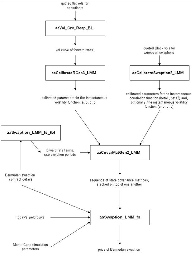
Figure 3:
Data flow through FINCAD functions in order to price a Bermudan swaption
using the LIBOR Market Model.
Assume the Bermudan swaption being valued has settlement
date of 14-Feb-2000, an effective date of 15-Mar-2000 and a maturity date of 15-Mar-2004. An accrual method of 30/360, no business day
adjustments and linear interpolation are used for all calculations. The fixed and floating payments are both
annual, the principal amount is 100, the fixed coupon is 5.0% and the swaption
is the right to receive fixed.
First we generate the rate terms and coupon periods using aaDateGen
with the following inputs:
aaDateGen
|
Argument |
Description |
Example Data |
Switch |
|
d_s |
settlement date |
14-Feb-2000 |
|
|
d_t |
terminating date |
15-Mar-2004 |
|
|
d_e |
effective date |
15-Mar-2000 |
|
|
d_f_cpn |
date of first coupon after effective date |
omitted |
|
|
d_l_cpn |
date of last coupon prior to terminating date |
omitted |
|
|
freq |
cash flow frequency |
1 |
annual |
|
hl |
holiday list |
empty (for simplicity) |
|
|
d_rul |
business day convention |
1 |
no date adjustment |
|
table_type |
table type |
2 |
two-column array |
The output rate terms and coupon periods are:
Output Table 1 – rate terms/coupon periods
|
Effective Date |
Terminating Date |
|
15-Mar-2000 |
15-Mar-2001 |
|
15-Mar-2001 |
15-Mar-2002 |
|
15-Mar-2002 |
15-Mar-2003 |
|
15-Mar-2003 |
15-Mar-2004 |
Given the coupon periods and rate terms, we build
the swap table:
t_1225 – swap table
|
rate eff date |
rate term date |
coupon eff date |
coupon term date |
NPA |
cpn |
margin |
ex flag |
ex fee |
|
15-Mar-2000 |
15-Mar-2001 |
15-Mar-2000 |
15-Mar-2001 |
100 |
5.0% |
0.0% |
1 |
0.0% |
|
15-Mar-2001 |
15-Mar-2002 |
15-Mar-2001 |
15-Mar-2002 |
100 |
5.0% |
0.0% |
1 |
0.0% |
|
15-Mar-2002 |
15-Mar-2003 |
15-Mar-2002 |
15-Mar-2003 |
100 |
5.0% |
0.0% |
1 |
0.0% |
|
15-Mar-2003 |
15-Mar-2004 |
15-Mar-2003 |
15-Mar-2004 |
100 |
5.0% |
0.0% |
1 |
0.0% |
We now generate the evolution periods
and forward rates for
aaSwaption_LMM_fs_tbl
|
Argument |
Description |
Example Data |
Switch |
|
d_v |
value date |
14-Feb-2000 |
|
|
swap_tbl |
swap table |
t_1225 (above) |
|
|
table_type |
table type |
1…2 |
period dates table or forward rate table |
The evolution periods (table_type = 1) and forward
rates (table_type = 2) from aaSwaption_LMM_fs_tbl are:
Output Table 2 – period dates table
|
Effective Date |
Terminating Date |
|
14-Feb-2000 |
15-Mar-2000 |
|
15-Mar-2000 |
15-Mar-2001 |
|
15-Mar-2001 |
15-Mar-2002 |
|
15-Mar-2002 |
15-Mar-2003 |
Output Table 3 –forward rate table
|
Effective Date |
Terminating Date |
|
15-Mar-2000 |
15-Mar-2001 |
|
15-Mar-2001 |
15-Mar-2002 |
|
15-Mar-2002 |
15-Mar-2003 |
|
15-Mar-2003 |
15-Mar-2004 |
Note that the list of forward rates in Output
Table 3 includes all rates from the swap table above (t_1225), because all of
these rates set in the future (i.e., after
the Value Date). Also note that there
are 4 rate evolution periods in Output Table 2.
To price the swaption, forward rates need to be evolved to each of the
rate effective dates. Rates also need to
be evolved to all coupon terminating dates (except the last one) because the swaption
is exercisable on these dates. These swaption
exercise dates coincide with the rate effective dates, so we need only consider
the rate effective dates when determining the rate evolution periods, which is
why there are 4 periods in Output Table 2.
The function aaCovarMatGen2_LMM
can be used to generate the sequence of covariance matrices required as an
input to aaSwaption_LMM_fs. Suppose that aaCalibrateSwaption2_LMM
has been used to calibrate the LMM to swaptions, with the 4-parameter linear-exponential
parametric form for instantaneous lognormal volatilities, the exponential form
for instantaneous correlations, and volatility scale factors set to 1 (see the Calibration
FINCAD Math Reference document).
Alternatively we could have used aCalibrateRCap3_LMM
to calibrate the instantaneous lognormal volatility parameters (![]() ), then used aaCalibrateSwaption2_LMM to calibrate the
instantaneous correlation parameters (
), then used aaCalibrateSwaption2_LMM to calibrate the
instantaneous correlation parameters (![]() and
and ![]() ). The calibrated
parameter values are assembled in Output Table 4.
). The calibrated
parameter values are assembled in Output Table 4.
Output Table 4 – Model Parameters
|
a |
b |
c |
d |
beta1 |
beta2 |
|
-0.02 |
0.3 |
2 |
0.16 |
0.1 |
0.1 |
Output Tables 2 through 4 are used by aaCovarMatGen2_LMM
to generate the covariance matrices for the Bermudan swaption. The complete list of inputs to aaCovarMatGen2_LMM
is shown below.
aaCovarMatGen2_LMM
|
Argument |
Description |
Example Data |
Switch |
|
d_v |
Valuation (settlement) date |
14-Feb-2000 |
|
|
period_date_tbl |
Table containing starting and end dates for a set of time
periods |
Output Table 2 (above) |
|
|
fwdrate_tbl |
Table containing effective and terminating dates for a set
of forward rates |
Output Table 3 (above) |
|
|
acc |
Day count convention |
4 |
30/360 |
|
model_vol |
Parameterization of instantaneous volatility |
1 |
4-parameter linear exponential |
|
model_cor |
Parameterization of instantaneous correlation |
1 |
2-parameter exponential |
|
model_parms |
Table containing values of all model parameters |
Output Table 4 (above) |
|
|
scalfac_tbl |
Volatility scale factor table for forward rates. |
1 |
|
Output Table 5 shows the sequence of four 4x4 covariance
matrices generated by aaCovarMatGen2_LMM, which is used to evolve
the 4 forward rates over the 4 time periods.
Output Table 5 – Covariance Matrix Sequence
|
0.00202425 |
0.00236746 |
0.00187570 |
0.00163840 |
|
0.00236746 |
0.00332062 |
0.00262800 |
0.00229292 |
|
0.00187570 |
0.00262800 |
0.00248774 |
0.00216844 |
|
0.00163840 |
0.00229292 |
0.00216844 |
0.00226080 |
|
0.00000000 |
0.00000000 |
0.00000000 |
0.00000000 |
|
0.00000000 |
0.03864862 |
0.03258181 |
0.02709047 |
|
0.00000000 |
0.03258181 |
0.03333816 |
0.02760589 |
|
0.00000000 |
0.02709047 |
0.02760589 |
0.02736581 |
|
0.00000000 |
0.00000000 |
0.00000000 |
0.00000000 |
|
0.00000000 |
0.00000000 |
0.00000000 |
0.00000000 |
|
0.00000000 |
0.00000000 |
0.03864862 |
0.03258181 |
|
0.00000000 |
0.00000000 |
0.03258181 |
0.03333816 |
|
0.00000000 |
0.00000000 |
0.00000000 |
0.00000000 |
|
0.00000000 |
0.00000000 |
0.00000000 |
0.00000000 |
|
0.00000000 |
0.00000000 |
0.00000000 |
0.00000000 |
|
0.00000000 |
0.00000000 |
0.00000000 |
0.03864862 |
Finally we call aaSwaption_LMM_fs. We select 2nd order polynomials as
basis functions and the 1st two moments of the interest rate curve
as regression variables (as described under Formulas
& Technical Details above).
We use all possible random factors, which in this case is 4 (the maximum
number of stochastic rates in any one period is 4) and we use 1000
t_43_32 – discount factor curve
|
grid date |
discount factor |
|
14-Feb-2000 |
1.00000000 |
|
15-Feb-2000 |
0.99986634 |
|
15-Aug-2000 |
0.97583485 |
|
15-Feb-2001 |
0.95212637 |
|
15-Aug-2001 |
0.92936652 |
|
15-Feb-2002 |
0.90678702 |
|
15-Aug-2002 |
0.88511098 |
|
15-Feb-2003 |
0.86360669 |
|
15-Aug-2003 |
0.84296283 |
|
15-Feb-2004 |
0.82248256 |
|
15-Aug-2004 |
0.80271444 |
|
15-Feb-2005 |
0.78321202 |
|
15-Aug-2005 |
0.76448994 |
|
15-Feb-2006 |
0.74591621 |
|
15-Aug-2006 |
0.72808566 |
|
15-Feb-2007 |
0.71039639 |
|
15-Aug-2007 |
0.69341491 |
|
15-Feb-2008 |
0.67656799 |
|
15-Aug-2008 |
0.66030689 |
|
15-Feb-2009 |
0.64426435 |
|
15-Aug-2009 |
0.62886370 |
|
15-Feb-2010 |
0.61358509 |
|
15-Aug-2010 |
0.59891781 |
|
14-Feb-2011 |
0.58439810 |
|
14-Feb-2012 |
0.55648080 |
|
14-Feb-2013 |
0.52982607 |
|
14-Feb-2014 |
0.50451573 |
|
14-Feb-2015 |
0.48041449 |
aaSwaption_LMM_fs
|
Argument |
Description |
Example Data |
Switch |
|
d_v |
value (settlement) date |
14-Feb-2000 |
|
|
swap_tbl |
swap table |
t_1225 (above) |
|
|
acc_pay |
accrual method for coupon periods |
4 |
30/360 |
|
acc_rate |
accrual method for rate terms |
4 |
30/360 |
|
df_crv |
discount factor curve |
t_43_32 (above) |
|
|
intrp |
interpolation method |
1 |
linear |
|
covar_mat |
covariance matrix |
Output Table 5 (above) |
|
|
num_fact |
maximum number of stochastic factors per period |
4 |
|
|
reg_var |
regression variables |
1 |
IR curve moments |
|
basis_fn |
basis functions |
1 |
polynomial |
|
num_rnd |
number of random trials |
1000.5 |
|
|
table_type |
table type |
1 |
price table |
The output price table, showing price (1st
row) and accuracy (2nd row) is:
Output Table 6 – price table
|
Option price |
Expected time of exercise (in years) |
Probability of exercise |
|
1.181049 |
2.447973 |
0.575075 |
|
0.113669 |
0.128543 |
0.037544 |
The 95% confidence interval for the option price is:
[1.181049 – 0.113669, 1.181049 + 0. 113669] = [1.067381, 1.294718].
Accuracy values can be made smaller by increasing
the number of
Related Functions
aaCalibrateRcap2_LMM,
aaCalibrateRcap3_LMM,
aaCalibrateSwaption2_LMM,
aaVol_Crv_Rcap_BL
LMM calibration
functions and caplet volatility bootstrapping function
aaCallSnowball_LMM_fs,
aaCallSnowball_LMM_LV_fs,
aaCallSnowball_LMM_fs_tbl
Snowball valuation
functions
aaSwaption_dgen,
aaSwaption_dgen_cf,
aaSwaption2_dgen,
aaSwaption2_dgen_cf,
aaSwaption_HW,
aaSwaption_BK,
aaSwaption2_HW,
aaSwaption2_BK,
aaSwaption_MF
Short-rate
tree-based Bermudan swaption valuation functions
aaCaplet_HW,
aaCaplet_BK,
aaCaplet_MF,
aaRcap_HW,
aaRcap_BK,
aaRcap_MF,
aaSwaption_eu_HW,
aaSwaption_eu_BK,
aaSwaption_eu_MF,
aaCalibrateRcap2_HW,
aaCalibrateRcap2_BK,
aaCalibrateRcap2_MF,
aaCalibrateSwaption2_HW,
aaCalibrateSwaption2_BK,
aaCalibrateSwaption2_MF
Short rate
calibration and calibration instrument pricing functions
References
[1]
Andersen, L. and Andreasen, J. (1998),
‘Volatility Skews and Extensions of the Libor Market Model’, Mathematical Finance, 7, 127-155.
[3]
Brigo, D. and Mercurio, F. (2001), Interest Rate Models, Theory and Practice,
[4]
[5]
[6]
Jaeckel, P. (2002), Monte
Carlo Methods in Finance,
[7]
Joshi, M. (2003), The
Concepts and Practice of Mathematical Finance,
[8]
Longstaff, F. and Schwartz, E. (2001), ‘Valuing
American Options by Simulation: A Simple Least Squares Approach’, The Review of Financial Studies, 14,
113-147.
[10] Muck,
M. (2003) ‘On the Similarity between Displaced Diffusion and Constant
Elasticity of Variance Market Models of the Term Structure’, German Finance
Association 11th Annual Meeting,
[14]
Rebonato, R. (2002) Modern
Pricing of Interest-Rate Derivatives, Princeton:
Disclaimer
With respect to this document,
FinancialCAD Corporation (“FINCAD”) makes no warranty either express or
implied, including, but not limited to, any implied warranty of merchantability
or fitness for a particular purpose. In no event shall FINCAD be liable to
anyone for special, collateral, incidental, or consequential damages in
connection with or arising out of the use of this document or the information
contained in it. This document should not be relied on as a substitute for your
own independent research or the advice of your professional financial,
accounting or other advisors.
This information is subject to change
without notice. FINCAD assumes no responsibility for any errors in this
document or their consequences and reserves the right to make changes to this
document without notice.
Copyright
Copyright © FinancialCAD Corporation 2008.
All rights reserved.