General Root Finding (_ix) Functions
Overview
The inputs to any “_ix”
function are the same as to the corresponding regular function, plus an
additional input table containing:
·
the method of solution
1 = Method of Bisection
2 = Brent’s method
·
the index of the sought parameter
·
the index of the output statistic (whose value
is known)
·
the desired (known) value of the output
statistic
·
the accuracy tolerance for the iterative
algorithm (defines when the solution is close enough)
·
the initial range (min/max) that contains the
solution
Both minimum
and maximum values of the initial range must adhere to the sought parameter's
restrictions. Valid inputs must be given
for all input parameters of the function, including the sought parameter
(although any valid input will do). The
sought parameter must be non-integer (e.g., not a switch or a date input) and
single-celled (i.e., not a table input).
The output table
contains:
·
the number of iterations performed
·
a code indicating whether the algorithm was
successful or not:
0 = solution was
found successfully
1 = invalid method
input (must be 1 or 2)
2 = no solution
was found
3 = took more than
50 iterations (to overcome this, try increasing the accuracy tolerance)
·
the solution (i.e., the value of the input
parameter)
·
the value of the function corresponding to the
found solution (should be approximately equal to the desired value)
It is useful
to understand the behavior of the regular function prior to use of its “_ix”
version by plotting the output statistic against the input parameter, as in the
examples below. This step is useful for
determining the initial range, and in understanding when the “_ix” function
might fail to find a solution in the given range for the given target
value. Several important issues
concerning the use of the root finding functions are described below.
Formulas & Technical Details
![]()
for some FINCAD
function ![]() with constant value of
the output statistic
with constant value of
the output statistic ![]() , for some unknown input parameter
, for some unknown input parameter ![]() . For example, one
might want to know the value of the implied volatility
. For example, one
might want to know the value of the implied volatility ![]() that gives an option’s
fair price
that gives an option’s
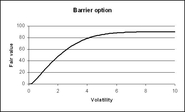
fair price ![]() . The knock-in call
fair value vs. volatility is illustrated in the following figure. It can be easily seen that the fair value of
$60 corresponds to an implied volatility of 2.6%, and so on.
. The knock-in call
fair value vs. volatility is illustrated in the following figure. It can be easily seen that the fair value of
$60 corresponds to an implied volatility of 2.6%, and so on.

Figure 1
The user has
to be sure that there is a solution which lies inside the specified
interval. In the example above (target
price $60), solving for the implied volatility within the interval, say 1% to
2%, would not find a root. Solving for a
fair value above $100 would also not find a root, for any interval of the
volatility. The function returns a
failure code in both cases.
There is a choice of
the Method of Bisection or Brent’s [1] Method. The
Bisection Method never fails to find a root if one exists, but it is slower to
converge than Brent’s. For most of the
output statistics of FINCAD functions there is a single root that either
Bisection or Brent method can easily find.
The Bisection Method algorithm computes the output statistic value at
the end points of the interval and at the middle point. It compares these three values and replaces
one of the end points with the middle one.
Because each iteration reduces the interval size in half, the number of
iterations required is proportional to the logarithm of the accuracy tolerance;
roughly 3 iterations are required for every extra decimal digit of the
solution. Brent’s method is faster than
the Bisection Method, and also guarantees to find the root if there is one in
the given interval. It employs an
inverse quadratic interpolation, which uses three prior points to fit an
inverse quadratic function (x as a quadratic
function of y) whose value at zero is taken
as the next estimate for the root x. Neither method requires an evaluation of the
function’s derivative.
Special attention
should be paid in the case of multiple roots. If the function has an even number of roots in
the given interval, the root finding algorithm returns an error (see more in Examples). If
the number of roots is odd (>1), one of the roots will be found. This situation however is unlikely to cause
confusion, since functions with such a behavior do not generally exist in the
FINCAD library. In addition, the
interval should not contain a discontinuity since the method may also fail.
FINCAD Functions
aaBarrier_ix(price_u,
ex, bar, d_v, d_exp, bar_type, rebate, vlt, rate_ann, cost_hldg, option_type, ix_parm_x)
aaBarrier_am_ix(price_u,
ex, bar, d_v, d_exp, bar_type, rebate, vlt, rate_ann, cost_hldg, option_type,
optimize, ix_parm_x)
aaBarrier_dbl_ix(d_v, d_exp,
price_u, ex, bar1, bar2, rebate_up, rebate_dn, vlt, rate_ann, cost_hldg, option_type,
optimize, option_style, ix_parm_x)
aaBarrier_dbl_bin_ix(d_v, d_exp,
price_u, ex, bar1, bar2, rebate_exp, rebate_up, rebate_dn, vlt, rate_ann, cost_hldg,
option_type, optimize, ix_parm_x)
aaBarrier_dbl_bin_dbltouch_ix(d_v, d_exp,
price_u, ex, bar1, bar2, bar_type, payoff, cash, vlt, rate_ann, cost_hldg, option_type,
dblTouch_stat,I x_parm_x)
aaBarrier_dbl_bin_hit_cash_ix(d_v, d_exp,
price_u, bar1, bar2, rebate_up, rebate_dn, rebate_exp, paytime_type, vlt, rate_ann,
cost_hldg, ix_parm_x)
aaBarrier_dbl_bin_mix_ix(d_v, d_exp,
price_u, ex, bar1, bar2, hit_order, bar_type, payoff, cash, vlt, rate_ann, cost_hldg,
option_type, ix_parm_x)
aaBarrier_dbl_bin_onetouch_ix(d_v, d_exp,
price_u, ex, bar1, bar2, bar_type, payoff, cash, vlt, rate_ann, cost_hldg, option_type,
ix_parm_x)
aaBarrier_dbl_dbltouch_ix(d_v, d_exp,
price_u, ex, bar1, bar2, bar_type, vlt, rate_ann, cost_hldg, option_type, dblTouch_stat,
ix_parm_x)
aaBarrier_dbl_mix_ix(d_v, d_exp,
price_u, ex, bar1, bar2, hit_order, bar_type, vlt, rate_ann, cost_hldg, option_type,
ix_parm_x)
aaBarrier_dbl_onetouch_ix(d_v, d_exp,
price_u, ex, bar1, bar2, bar_type, vlt, rate_ann, cost_hldg, option_type, ix_parm_x)
aaBarrier_eu_ix(price_u,
ex, bar, d_v ,d_exp, bar_type, rebate, vlt, rate_ann, cost_hldg, option_type, ix_parm_x)
aaBinary_bar_hit_asset_ix(price_u,
bar, d_v, d_exp, bar_type, paytime_type, vlt, rate_ann, cost_hldg, ix_parm_x)
aaBinary_bar_hit_cash_ix(price_u,
bar, d_v, d_exp, bar_type, cash, paytime_type, vlt, rate_ann, cost_hldg, ix_parm_x)
aaBinary_bar_in_asset_ix(price_u,
ex, bar, d_v, d_exp, bar_type, vlt, rate_ann, cost_hldg, option_type, ix_parm_x)
aaBinary_bar_in_cash_ix(price_u,
ex, bar, d_v, d_exp, bar_type, cash, vlt, rate_ann, cost_hldg, option_type, ix_parm_x)
aaBinary_bar_nohit_asset_ix(price_u,
bar, d_v, d_exp, bar_type, vlt, rate_ann, cost_hldg, ix_parm_x)
aaBinary_bar_nohit_cash_ix(price_u,
bar, d_v, d_exp, bar_type, cash, vlt, rate_ann, cost_hldg, ix_parm_x)
aaBinary_bar_out_asset_ix(price_u,
ex, bar, d_v, d_exp, bar_type, vlt, rate_ann, cost_hldg, option_type, ix_parm_x)
aaBinary_bar_out_cash_ix(price_u,
ex, bar, d_v, d_exp, bar_type, cash, vlt, rate_ann, cost_hldg, option_type, ix_parm_x)
aaFX_Barrier_am_ix(amount,
princ_curr, FX_unit, FX_rate, asset_type, FX_ex, FX_bar, bar_type, d_exp, d_v, vlt,
intrp, df_prim, df_sec, option_type, rebate, optimize, ix_parm_x)
aaFX_Barrier_eu_ix(amount,
princ_curr, FX_unit, FX_rate, asset_type, FX_ex, FX_bar, bar_type, d_exp, d_v, vlt,
intrp, df_prim, df_sec, option_type, rebate, ix_parm_x)
aaFX_Binary_bar_hit_cash_ix(FX_rate,
FX_bar, princ_curr, FX_unit, d_v, d_exp, vlt, bar_type, cash, paytime_type, intrp,
df_prim, df_sec, asset_type, amount, ix_parm_x)
aaFX_Binary_bar_in_cash_ix(FX_rate,
FX_ex, FX_bar, princ_curr, FX_unit, d_v, d_exp, vlt, bar_type, cash, intrp, df_prim,
df_sec, option_type, asset_type, amount, ix_parm_x)
aaFX_Binary_bar_nohit_cash_ix(FX_rate,
FX_bar, princ_curr, FX_unit, d_v, d_exp, vlt, bar_type, cash, intrp, df_prim, df_sec,
asset_type, amount, ix_parm_x)
aaFX_Binary_bar_out_cash_ix(FX_rate,
FX_ex, FX_bar, princ_curr, FX_unit, d_v, d_exp, vlt, bar_type, cash, intrp, df_prim,
df_sec, option_type, asset_type, amount, ix_parm_x)
aaQuanto_Barrier_am_ix(price_ufor,
ex_for, FX_fix, barrier, d_v, d_exp, barrier_type, rebate, vlt_u, vlt_FX, corr,
rate_for_ann, rate_dom_ann, cost_hldg, option_type, optimize, ix_parm_x)
aaQuanto_Barrier_dbl_ix(d_v, d_exp,
price_ufor, ex_for, FX_fix, bar1, bar2, rebate_up, rebate_dn, vlt_u, vlt_FX, corr,
rate_for_ann, rate_dom_ann, cost_hldg, option_type, optimize, option_style, ix_parm_x)
aaQuanto_Barrier_dbl_bin_ix(d_v, d_exp,
price_ufor, ex_for, FX_fix, bar1, bar2, rebate_exp, rebate_up, rebate_dn, vlt_u,
vlt_FX, corr, rate_for_ann, rate_dom_ann, cost_hldg, option_type, optimize, ix_parm_x)
aaQuanto_Barrier_eu_ix(price_ufor,
ex_for, FX_fix, barrier, d_v, d_exp, barrier_type, rebate, vlt_u, vlt_FX, corr,
rate_for_ann, rate_dom_ann, cost_hldg, option_type, ix_parm_x)
aaQuanto_Binary_hit_asset_ix(price_ufor,
barrier, FX_fix, d_v, d_exp, barrier_type, paytime_type, vlt_u, vlt_FX, corr, rate_for_ann,
rate_dom_ann, cost_hldg, ix_parm_x)
aaQuanto_Binary_hit_cash_ix(price_ufor,
barrier, FX_fix, d_v, d_exp, barrier_type, cash, paytime_type, vlt_u, vlt_FX, corr,
rate_for_ann, rate_dom_ann, cost_hldg, ix_parm_x,)
aaQuanto_Binary_in_asset_ix(price_ufor,
ex_for, FX_fix, barrier, d_v, d_exp, barrier_type, vlt_u, vlt_FX, corr, rate_for_ann,
rate_dom_ann, cost_hldg, option_type, ix_parm_x)
aaQuanto_Binary_in_cash_ix(price_ufor,
ex_for, FX_fix, barrier, d_v, d_exp, barrier_type, cash, vlt_u, vlt_FX, corr, rate_for_ann,
rate_dom_ann, cost_hldg, option_type, ix_parm_x)
aaQuanto_Binary_nohit_asset_ix(price_ufor,
barrier, FX_fix, d_v, d_exp, barrier_type, vlt_u, vlt_FX, corr, rate_for_ann,
rate_dom_ann, cost_hldg, ix_parm_x)
aaQuanto_Binary_nohit_cash_ix(price_ufor,
barrier, FX_fix, d_v, d_exp, barrier_type, cash, vlt_u, vlt_FX, corr, rate_for_ann,
rate_dom_ann, cost_hldg, ix_parm_x)
aaQuanto_Binary_out_asset_ix(price_ufor,
ex_for, FX_fix, barrier, d_v, d_exp, barrier_type, vlt_u, vlt_FX, corr, rate_for_ann,
rate_dom_ann, cost_hldg, option_type, ix_parm_x)
aaQuanto_Binary_out_cash_ix(price_ufor,
ex_for, FX_fix, barrier, d_v, d_exp, barrier_type, cash, vlt_u, vlt_FX, corr, rate_for_ann,
rate_dom_ann, cost_hldg, option_type, ix_parm_x)
Description of Inputs
ix_parm_x
|
Column # |
Label |
Description |
|
1 |
Method |
1=Bisection or 2=Brent |
|
2 |
Input index |
Index of the input parameter |
|
3 |
Stats index |
Index of the output statistic |
|
4 |
Stats value |
The desired (target) value of the output statistic |
|
5 |
Accuracy |
Accuracy tolerance of the sought parameter |
|
6 |
Input min |
Lower limit of the initial interval for the sought
parameter |
|
7 |
Input max |
Upper limit of the initial interval for the sought
parameter |
Description of Outputs
|
Label |
Description |
|
|
1 |
number of iterations
used |
|
|
2 |
method converged |
status code 0 = solution was found
successfully 1 = invalid method
input (must be 1 or 2) 2 = no solution was
found 3 = took more than 50
iterations |
|
3 |
found parameter |
solution; i.e., the
value of the input parameter |
|
4 |
f(parameter) |
value of the output
statistic for the found parameter |
Examples
We consider two examples: a European and an American barrier
option. We want to find the barrier that
would give a certain fair value of the option.
The first option is a European knock-in call, for which we use the
FINCAD function aaBarrier.
The inputs are the price of the underlying security $100, the exercise
price $100, and the barrier arbitrarily set to $90. The option is valued on January 13, 2001 with
an exercise date of January 24, 2002. We
set the risk-free rate to 6%, with zero holding costs.
Suppose the option’s fair price is $5. We enter parameters for the root finding in
table t_1122. The method used is 1
(Bisection), the input index is 3 (since the barrier is the third argument of aaBarrier),
the statistic index is 1 (= fair value), and the accuracy tolerance of the
sought value is $0.01. Special care
should be taken with the minimum and maximum values of the sought parameter as
illustrated below.
aaBarrier_ix
|
Argument |
Description |
Example Data |
Switch |
|
price_u |
underlying price |
100 |
|
|
ex |
exercise price |
100 |
|
|
bar |
barrier |
90 |
|
|
d_v |
value (settlement) date |
13-Jun 2001 |
|
|
d_exp |
expiry date |
24-Jan 2002 |
|
|
bar_type |
barrier type |
1 |
knock-in |
|
rebate |
rebate if barrier is hit (knock out) |
0 |
|
|
vlt |
volatility rate |
20.0% |
|
|
rate_ann |
rate – annual – Actual/365 |
6.0% |
|
|
cost_hldg |
holding cost – annual – Actual/365 |
0.0% |
|
|
option_type |
option type |
1 |
call |
t_1122 - root finding parameters
|
method |
input index |
stats index |
stats value |
accuracy |
input min |
input max |
|
1 |
3 |
1 |
5 |
0.01 |
50 |
100 |
|
Bisection |
barrier |
fair value |
$5.00 |
$.01 |
from $50 |
to $100 |
Results: table_1132 - aaBarrier_ix
|
number of iterations used |
method converged? (0=true,else=false) |
found parameter |
f(parameter) |
|
13 |
0 |
97.44 |
4.99 |
|
13 iterations
used |
unique solution
found |
the solution |
» target price |

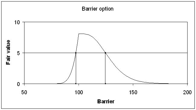
Figure 2
As can be seen in the plot above, a fair value of
$5 (for that matter of any value less than $8.07 and greater than $0) has two
roots which correspond to two different call options – up-in and down-in. In other words, two different barrier values
give the same desired fair value. If the
initial range was $70 to $150, then the root finding would fail since there is
an even number (2) of solutions. By
examining the plot, one can identify that the first solution lies between $70
and $110, and the second one between $110 and $150. Choosing these two ranges produces two
results: $97.44 and $124.66; each one
gives the correct price for an up-in or down-in call respectively.
Caution should be exercised when dealing with functions
whose computational engine is a binomial tree, such as American-style barrier
options. Due to the discrete nature of binomial
trees the output values also have discrete values when there is a barrier. This introduces noise to the shape of the fair
price curve, especially if a low level of optimization is chosen (too few time
steps in the binomial tree). In this
case the root finding algorithm may only succeed for a large accuracy
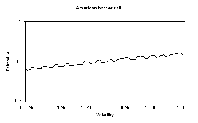
tolerance. To illustrate this point, the
fair value of an American barrier option is plotted below. This is a down-and-out American call option. The underlying security is $100, the exercise
price is $100, and the barrier is (arbitrarily) at $90. The option is valued on January 1, 2003 with
an exercise date of January 1, 2004. The
risk-free rate is 10%, with zero holding costs, and the volatility is 25%. With a low optimization level (e.g., 2), the
fair value plot has significant noise at the plot scale.

Figure 3
The root solving problem becomes ambiguous if the
requested accuracy tolerance is too strict.
By choosing different initial ranges for the volatility, for the same
desired output value one can obtain different values for the sought parameter. For example, if the target value for the Fair
Value is 11.00 in the above plot, then there are at least 5 possible solutions
for the volatility. This issue appears
similar but is different in nature from the two-root problem discussed
previously, since the solutions may now differ by less than the accuracy
tolerance. This problem can be solved by
either increasing the optimization level in the binomial tree, or by relaxing
the accuracy tolerance.
Related Functions
|
Original Function |
Inverse Function |
References
Disclaimer
With respect
to this document, FinancialCAD Corporation (“FINCAD”) makes no warranty either
express or implied, including, but not limited to, any implied warranty of
merchantability or fitness for a particular purpose. In no event shall FINCAD
be liable to anyone for special, collateral, incidental, or consequential
damages in connection with or arising out of the use of this document or the
information contained in it. This document should not be relied on as a
substitute for your own independent research or the advice of your professional
financial, accounting or other advisors.
This
information is subject to change without notice. FINCAD assumes no
responsibility for any errors in this document or their consequences and
reserves the right to make changes to this document without notice.
Copyright
Copyright ©
FinancialCAD Corporation 2008. All rights reserved.