![]()
Tax-Exempt (Municipal) Swap Curve
Overview
A BMA swap is an interest rate swap in which the payments
of one leg are variable and are based upon fixings of the US SIFMA Municipal
Swap Index (formerly the BMA Municipal Swap Index or “BMA Index”). This index is produced weekly, reflecting the
average rate of issues of tax-exempt variable-rate debt, and serves as a
benchmark floating rate in municipal swap transactions. The BMA index is usually 65%-70% of its
taxable equivalent 1-month Libor. This
ratio is subject to tax-risk, i.e., the risk that marginal tax rates will
change or that there will be revisions to the US Tax Code.
The BMA Swap Curve represents the expected future values
of the BMA index, where expectations are taken in the corresponding forward
probability measure; the forward rates that are encoded in the curve can be
used to calculate expected future cash-flows for the purpose of valuing the BMA
leg. Similar to other curve generation processes, the BMA Swap Curve is
generated using a set of quoted cash rates and par rates for BMA fixed/floating
swaps. Another important input is the risk-free discount factor curve (usually
the Libor curve), which is used to calculate the present value of expected
future cashflows. The par rate for a BMA
fixed/floating swap of a particular maturity (e.g., 10 years) can be derived
from the BMA Basis factor for that maturity (e.g., 75%) and the corresponding
Libor swap rate. A BMA Basis factor of
75% means that a BMA/Libor basis swap, in which one leg pays 75% of Libor, and
the other leg pays BMA, is a par swap.
Thus, if the 10Y Libor swap rate (for a 10Y fixed/floating Libor swap)
is, say, 4%, then the par rate for a BMA fixed/floating swap is 75% ´ 4% = 3%.
Bootstrapping starts with the shortest term swap and steps
through them all in ascending order of maturity. At every step, forward rates inferred from
the preceding swaps are considered as known, and subsequent forward rates are
constrained to recover the price of the current swap. Refer to the Interest Rate Curve Generation FINCAD
Math Reference document for more
information on curve generation, and Floating
Rate Notes with Averaging (muni / tax-exempt market) FINCAD
Math Reference document for how to
value the BMA leg of a BMA swap. When valuing
the BMA leg, the BMA Swap Curve is intended to be used as the “accruing curve” (used
to calculate expected cashflows from its implied forward rates). The Libor
curve would typically be used as the “discounting curve”. The BMA swap Curve is not
intended to be used as a “discounting curve”; the 2-column format [date,
discount_factor] is merely a representation to encode the forward rates in a
way that is consistent with the format of other FINCAD interest rate curves.
Formulas and Technical Details
The function aaSwap_crv_avg
takes in a table of swap rates and/or basis factors; the latter are the scaling
factors to apply to the internally-calculated LIBOR swap rates. Each row in the table that has a basis factor
as the rate will be converted to a BMA swap rate using the function aaParSwap3
with the inputs of the fixed leg payment frequency and daycount equal
to the BMA swap's fixed leg (i.e., as specified by the freq_fixed and acc_fix
inputs, respectively). For example, if
the frequency of the BMA swap's fixed leg is specified as quarterly, then
internally the quarterly LIBOR swap rate is calculated, multiplied by the basis
factor, and used as the BMA swap rate. If
a different frequency and daycount for the basis factor is needed by the user
then the scaled swap rate should be calculated externally, and passed into aaSwap_crv_avg
as swap rates.
The bootstrapping process iterates through the given par
rates for BMA fixed/floating swaps, using the rules stated below, and outputs
discount factors and optionally forward rates. Note that the discount factor curve for
discounting (i.e., the Libor curve) is already known, and therefore it is only
necessary to build a curve that encodes implied forward rates.
The function aaSwap_crv_avg provides
a choice of three bootstrapping methods for building BMA curves, Linear Swap
Rates, Constant Forward Rates, and Quadratic Forward Rates. The last method
(Quadratic Forward Rates) give rise to the smoothest profiles for the forward
rates, and is the recommended method.
Linear Swap Rates
In this method a set of hypothetical swaps are created
that mature on each payment date of each of the given swaps. The par swap rate for each of these
hypothetical swaps is obtained by linear interpolation of the given swap rates,
based on the maturity date. The
algorithm steps through each hypothetical swap, in order of maturity. At each step the new swap has precisely one
more payment than the previous swap; the forward rates spanning this extra
payment period are calculated by assuming that they all have the same value.
In other words, it is assumed that the rate for all forward
periods (i.e., for each week in the case of the BMA index) spanning any two consecutive
payment dates are the same. This value
is determined by ensuring that the value of the floating leg equals that of the
fixed leg when the coupon equals the interpolated par swap rate.
For example, suppose that
·
today’s date is 29-May-2006,
·
the payment frequency of the BMA leg is quarterly,
·
the par swap rate for a maturity of 29-May-2007 is given as 5.72%,
·
the par swap rate for a maturity of 29-May-2008 is given as 5.80%, and
·
the forward BMA rates spanning the period
29-May-2006 to 29-May-2007 have been calculated by prior steps in the
algorithm.
The first step is to linearly interpolate a par
swap rate for a hypothetical maturity of 29-Aug-2007, which is the next payment
date after 29-May-2007. The interpolated
result is 5.74%. This hypothetical swap rate is used to calculate the weekly forward
rates spanning 29-May-2007 to 29-Aug-2007, assuming that the rates for all 13 or
14 forward periods within this 3-month payment period are equal to each other. The next step would be to use the interpolated
swap rate of 5.76% for a maturity of 29-Nov-2007 to calculate the 13 or 14
weekly forward rates spanning 29-Aug-2007 to 29-Nov-2007, assuming that they
are all equal. And so on.
Unfortunately the curves generated this way often have
saw-tooth shaped forward rate profiles. The following two methods overcome this
problem and generate curves with smoother forward rate profiles.
Constant Forward Rates
In this method, it is assumed that the rates for all the forward
periods spanning any two given swap maturities are the same.
For example, in the above example, it is assumed that the
rates for all weekly forward periods spanning 29-May-2007 to 29-May-2008 (about
53 of them) are equal to each other. Using this assumption, it is possible to directly
calculate the common forward rate that is consistent with the 5.80% par swap
rate.
This method will give rise to a staircase shaped forward
rate profile, comprised of a series of horizontal segments with vertical jumps
at each given swap maturity.
Quadratic Forward Rates
This method further improves the Constant Forward Rates Method
by smoothing out the discontinuities in the forward rate profile. The first step is to build a curve using the
Constant Forward Rates Method. The second step creates a sequence of parabolic
segments for the forward rate profile.
The parabolic segments match at each of the given swap maturities; i.e.,
part-way up the vertical jumps of the Constant Forward Rates Method. The
vertical coordinates of the match points are calculated as a function of the
height of each horizontal segment of the Constant Forward Rates Method. The parameters of each parabolic segment are chosen
to ensure that the smoothed curve is consistent with the input swap rates, and also
that the whole curve is continuous. The
end result is a curve whose forward rate profile is piecewise quadratic and
continuous (no jumps).
FINCAD Function
aaSwap_crv_avg(d_v,
cash_crv, swapcrv_bma_tbl, freq_fixed, drul_fix, acc_fix, freq_fl, drul_fl, acc_flt,
d_reset_cycle, reset_freq, d_rul_reset, acc_rt, reset_mktdays, rate_reset, hl, df_crv_disc,
intrp, rate_use, method_boot, output_type)
Calculates an accruing curve that implies forward rates
for the Municipal Swap Index, given a discounting (LIBOR) curve and par rates
(or basis factors) of tax-exempt municipal swaps whose floating leg payments
are based upon the average index rate.
Description of Inputs
|
Argument |
Description |
|
d_v |
value (settlement) date |
|
cash_crv |
cash/deposit rates |
|
swapcrv_bma_tbl |
par swap rates (or basis factors) |
|
freq_fixed |
frequency of fixed leg payments |
|
drul_fix |
business day adjustment for fixed leg payments |
|
acc_fix |
accrual method for fixed leg payments |
|
freq_fl |
frequency of floating leg payments |
|
drul_fl |
business day adjustment for floating leg payments |
|
acc_flt |
accrual method for floating leg payments |
|
d_reset_cycle |
reset cycle date |
|
reset_freq |
reset frequency |
|
d_rul_reset |
business day adjustment for reset dates |
|
acc_rt |
accrual method for reset/forward rates |
|
reset_mktdays |
number of business days prior to the rate effective date
that the index is fixed |
|
rate_reset |
current value of index |
|
hl |
holiday list |
|
df_crv_disc |
discount curve (LIBOR) |
|
intrp |
interpolation method |
|
rate_use |
rate tables to be used |
|
method_boot |
bootstrapping method: 1 = linear swap rates (constant forwards between swap
payments) 2 = constant forward rates (constant forwards between swap
maturities) 3 = quadratic forward rates |
|
output_type |
output curve type |
Description of Outputs
|
Table type |
Output |
|
1 |
discount factor curve |
|
2 |
discount factor and forward curve |
|
3 |
discount factor curve (monthly points) |
|
4 |
discount factor and forward curve (monthly points) |
|
5 |
discount factor curve (quarterly points) |
|
6 |
discount factor and forward curve (quarterly points) |
For Table Type 1 or 2, the function gives
discount factors for each forward rate effective date. When the reset frequency
is high, e.g., weekly, the output curve can be very long. The other table types
are provided for shorter curves, although this comes at a cost of interpolation
errors. For example, Table Type 5 would
give a discount factor curve that will only show discount factors on the dates
cycled quarterly from the maturity of the longest given swap. With a shortened
discount factor curve a round trip may not be achieved for par swaps, because
of the need for interpolation; i.e., when the curve is used to value the given
par swaps, the value may not be exactly zero.
Example
Suppose that money market rates and the basis factors are given
as follows:
Deposit rates
|
effective date |
terminating date |
rate |
rate quotation basis |
accrual method for
coupons |
use this point (0 =
no, 1 = yes) |
|
3-Dec-2006 |
4-Dec-2006 |
0.500% |
7 |
4 |
1 |
Swap rates
|
effective date |
terminating date |
rate or factor |
use this point |
swap rate or base
factor |
|
3-Dec-2006 |
3-Dec-2007 |
62.00% |
1 |
2 |
|
3-Dec-2006 |
3-Dec-2008 |
71.60% |
1 |
2 |
|
3-Dec-2006 |
3-Dec-2009 |
72.20% |
1 |
2 |
For the purposes of this example, the payment
frequency of the fixed leg and floating leg of the given swaps is quarterly,
and the reset frequency is weekly. Suppose further that the Libor curve (for
discounting) is given as follows:
Libor Curve (for discounting)
|
grid date |
discount factor |
|
3-Dec-2006 |
1 |
|
11-Dec-2006 |
0.999708 |
|
1-Jan-2007 |
0.998922 |
|
… |
… |
|
7-Dec-2013 |
0.758813 |
|
5-Dec-2014 |
0.717608 |
|
3-Dec-2015 |
0.676827 |
The following set of inputs is used to call aaSwap_crv_avg
using two different bootstrapping methods, Constant Forward Rates, and
Quadratic Forward Rates:
aaSwap_crv_avg
|
Argument |
Description |
Example data |
Switch |
|
d_v |
value (settlement) date |
3-Dec-2006 |
|
|
cash_crv |
cash/deposit rates |
see above |
|
|
swapcrv_bma_tbl |
par swap rates (or basis factors) |
see above |
|
|
freq_fixed |
frequency of fixed leg payments |
3 |
quarterly |
|
drul_fix |
business day adjustment for fixed leg payments |
2 |
next good business day |
|
acc_fix |
accrual method for fixed leg payments |
2 |
actual/360 |
|
freq_fl |
frequency of floating leg payments |
3 |
quarterly |
|
drul_fl |
business day adjustment for floating leg payments |
2 |
next good business day |
|
acc_flt |
accrual method for floating leg payments |
2 |
actual/360 |
|
d_reset_cycle |
reset cycle date |
6-Feb-2006 |
|
|
reset_freq |
reset frequency |
6 |
weekly |
|
d_rul_reset |
business day adjustment for reset dates |
1 |
no date adjustment |
|
acc_rt |
accrual method for reset/forward rates |
2 |
actual/360 |
|
reset_mktdays |
number of business days prior to the rate effective date
that the index is fixed |
0 |
|
|
rate_reset |
current value of index |
0.02 (or 2%) |
|
|
hl |
holiday list |
See below |
|
|
df_crv_disc |
discounting curve (LIBOR) |
See above |
|
|
intrp |
interpolation method |
1 |
linear |
|
rate_use |
rate tables to be used |
2 |
use both swap rates and cash rates |
|
method_boot |
bootstrapping method |
2 and 3 |
constant forward rates and quadratic forward rates |
|
output_type |
output curve type |
2 |
discount factor and forward curve |
|
holiday date |
|
1-Jan-2007 |
|
1-Jan-2008 |
The results using Constant Forward Rates are as
follows:
Results: Constant Forward Rates
|
Date |
Discount Factor |
Forward Rate |
|
3-Dec-2006 |
1 |
0.500000% |
|
4-Dec-2006 |
0.999986111 |
0.500000% |
|
11-Dec-2006 |
0.9998889 |
0.500000% |
|
18-Dec-2006 |
0.999712698 |
0.906441% |
|
25-Dec-2006 |
0.999536527 |
0.906441% |
|
… |
… |
… |
|
3-Dec-2007 |
0.99094208 |
0.906441% |
|
10-Dec-2007 |
0.990604178 |
1.754265% |
|
17-Dec-2007 |
0.990266391 |
1.754265% |
|
... |
... |
... |
|
8-Dec-2008 |
0.973191132 |
1.754265% |
|
15-Dec-2008 |
0.972667287 |
2.769765% |
|
22-Dec-2008 |
0.972143724 |
2.769765% |
|
... |
... |
... |
|
23-Nov-2009 |
0.947341346 |
2.769765% |
|
30-Nov-2009 |
0.946831416 |
2.769765% |
|
7-Dec-2009 |
0.94632176 |
2.769765% |
The results using Quadratic Forwards are as
follows:
Results: Quadratic
Forwards
|
Date |
Discount Factor |
Forward Rate |
|
3-Dec-2006 |
1 |
0.500000% |
|
4-Dec-2006 |
0.999986111 |
0.500000% |
|
11-Dec-2006 |
0.9998889 |
0.500000% |
|
18-Dec-2006 |
0.999788828 |
0.514763% |
|
25-Dec-2006 |
0.999685887 |
0.529580% |
|
1-Jan-2007 |
0.999580065 |
0.544452% |
|
8-Jan-2007 |
0.999471355 |
0.559378% |
|
15-Jan-2007 |
0.999359745 |
0.574359% |
|
22-Jan-2007 |
0.999245228 |
0.589394% |
|
29-Jan-2007 |
0.999127792 |
0.604483% |
|
5-Feb-2007 |
0.999007429 |
0.619626% |
|
12-Feb-2007 |
0.998884128 |
0.634824% |
|
19-Feb-2007 |
0.998757882 |
0.650076% |
|
26-Feb-2007 |
0.998628679 |
0.665382% |
|
5-Mar-2007 |
0.998496512 |
0.680743% |
|
12-Mar-2007 |
0.998361369 |
0.696158% |
|
19-Mar-2007 |
0.998223243 |
0.711628% |
|
26-Mar-2007 |
0.998082123 |
0.727152% |
|
2-Apr-2007 |
0.997938002 |
0.742730% |
|
… |
… |
… |
|
9-Feb-2009 |
0.969017841 |
2.500908% |
|
16-Feb-2009 |
0.968542469 |
2.524177% |
|
23-Feb-2009 |
0.968063055 |
2.546899% |
|
2-Mar-2009 |
0.967579708 |
2.569072% |
|
9-Mar-2009 |
0.967092538 |
2.590699% |
|
16-Mar-2009 |
0.966601654 |
2.611778% |
|
23-Mar-2009 |
0.966107164 |
2.632309% |
|
30-Mar-2009 |
0.965609176 |
2.652293% |
|
… |
… |
… |
|
12-Oct-2009 |
0.950680324 |
2.989555% |
|
19-Oct-2009 |
0.950127254 |
2.993662% |
|
26-Oct-2009 |
0.949573849 |
2.997220% |
|
2-Nov-2009 |
0.949020211 |
3.000232% |
|
9-Nov-2009 |
0.948466442 |
3.002695% |
|
16-Nov-2009 |
0.947912643 |
3.004612% |
|
23-Nov-2009 |
0.947358915 |
3.005980% |
|
30-Nov-2009 |
0.94680536 |
3.006802% |
|
7-Dec-2009 |
0.946252078 |
3.007075% |
Below is a graph of the forward curves produced using
both methods:
Results: Quadratic
Forwards and Constant Forward Rates
|
|
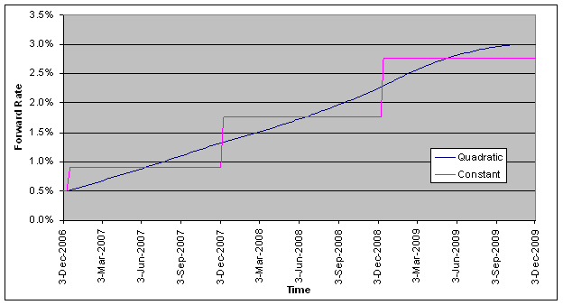
The staircase profile is evident for the curve produced
using Constant Forward Rates. Setting the bootstrapping method to “quadratic
forward rates” will result in a smoother profile of forward rates. The workbook ”Averaging Swap Curve”, that is
shipped with FINCAD XL, contains plots of the resulting forward rates, and is a
good tool for comparing the different methods and switch settings.
References
[1]
Floating Rate Notes with
Averaging (muni / tax-exempt market) FINCAD Math Reference document.
[2]
Interest
Rate Curve Generation FINCAD
Math Reference document.
Disclaimer
With respect to this document,
FinancialCAD Corporation (“FINCAD”) makes no warranty either express or
implied, including, but not limited to, any implied warranty of merchantability
or fitness for a particular purpose. In no event shall FINCAD be liable to
anyone for special, collateral, incidental, or consequential damages in
connection with or arising out of the use of this document or the information
contained in it. This document should not be relied on as a substitute for your
own independent research or the advice of your professional financial,
accounting or other advisors.
This information is subject to change
without notice. FINCAD assumes no responsibility for any errors in this
document or their consequences and reserves the right to make changes to this
document without notice.
Copyright
Copyright © FinancialCAD Corporation
2008. All rights reserved.