
Option Pricing from the Smile using Local Volatility
Overview
At least since the crash of 1987, the market implied
volatilities of equity options have exhibited a distinct “skew” structure. Deep out-of-the-money puts generally trade at
higher implied volatilities than out-of-the-money calls, reflecting the
market’s appetite for insurance against stock prices falling. Other types of options exhibit a volatility
“smile”, reflecting traders’ views on the likelihood of extreme movements in
exchange rates. We will use the term
“volatility smile” more loosely, to refer to any variation (smile, skew, frown,
etc) of implied volatility with strike price.
In addition to this variation with strike price, the implied volatility
of traded options generally also varies with the option maturity – the
volatility term structure – and so one often talks of an implied volatility
surface.
Arguably the most important problem in the theory of
options pricing is to take account of these market observations; in particular
to reconcile this structure of observed volatilities with the Black-Scholes
model [2] of option pricing used by traders to quote option
prices. If this model were correct in
its assumption that the underlying asset undergoes a lognormal Brownian motion
with a constant volatility, then all options written on that asset would trade
at the same implied volatility. Despite
the fact that they do not, the Black-Scholes formula remains a convenient tool
with which to measure the worth of an option.
Once one recognizes the deficiencies of the Black-Scholes framework,
however, it becomes clear that the implied volatility is really only the “… the
wrong number to put in the wrong formula to obtain the right price of plain vanilla
options” [16].
Although it is easy to modify the Black-Scholes model to
take account of the term structure of implied volatilities, the variation with
strike price – the volatility smile – is much harder to deal with. One of the concepts used to cope with this
problem is that of local volatility, as discussed originally by Dupire [8], Derman and Kani [6] and Rubenstein [17] in the context of the binomial model of option
pricing.
The constant volatility of the Black-Scholes model
corresponds to the assumption that the underlying asset follows a lognormal
stochastic process. As the name
suggests, local volatility can be thought of as taking this constant
volatility, and replacing it with a function which depends locally both on time
and on the value of the underlying asset.
The lognormal property is thus no longer true within the local
volatility framework. Rather the goal is
to determine the correct underlying process from the market-observed smile.
Given an implied volatility surface for European options written
on some asset, it is possible to determine the corresponding local volatility
function (i.e., local volatility as a function of time and underlying price) and
so indirectly determine the stochastic process driving the evolution of the
underlying asset. Various numerical
techniques can then be used in conjunction with the local volatility function
to price other options (say a European option with a different strike price, or
an American option, on the same asset).
In theory, this process ensures that the price of the latter American
option is “calibrated” to the prices of the European options taken from the
market.
In practice, one does not have access to a set of European
options with a complete range of strike prices and/or maturities, so there are
interpolation issues in the modeling of the implied volatility surface. The topic is an area of ongoing research, and
various methods have been discussed in the literature (see, e.g., [9] and [16]). We use a smoothing
technique as discussed in [5] and [10] which will be described in further detail below. This gives rise to a relatively well-behaved
local volatility function, which we use in conjunction with finite difference
methods, along the lines of [1], to price options “from the smile”.
The FINCAD functions described here allow European and
American options to be priced directly from the smile, and to examine the
associated local volatility function.
All the functions described here take an implied volatility surface as
their starting point. For details on how
to price options using the local volatility function as a starting point, see
the Option Pricing using a Local Volatility
Model FINCAD Math Reference document.
Following [9], FINCAD also provides a utility function to back out
the (risk-neutral) probability density function of the underlying asset, from
the market-observed volatility smile for options written on that asset. The first few moments (mean, variance, skew
and kurtosis) of the distribution are also computed.
Formulas & Technical Details
Basic Theory
The local volatility function is defined through the
process governing movements of an underlying asset price. Given a drift  and a local
volatility function[1]
 , movements of an asset
 are defined through
the Itô stochastic process[2]:
 ,
where  is a standard Brownian
motion, and the drift and local volatility can in general be arbitrary functions[3] of and
 . Using
standard arguments [14], the corresponding no-arbitrage partial differential
equation (PDE) for the price,
 , of an option written on the underlying asset is:
 ,
Equation 1
where, at least in the world of equity derivatives,  and
 are respectively the
continuously compounded risk-free interest rate and dividend yield per
annum. The fact that the drift does not
appear is the essence of the theory of risk-free pricing, and effectively
allows us to take
 , which we will always do.
This framework can be used to value various options, not
just those written on equities. To value
options on stock indices, take to be the index value,
and to be the dividend
yield on the index. To value options on
futures, take to be the futures
price and set  , since the effective return on the future is equal to
the risk-free rate. And to value FX
options, take to be the FX rate, to be the domestic
risk-free rate and to be the foreign
risk-free rate.
Equation
1 is the backward Kolmogorov equation. As shown by Dupire [8] (see also [6] and [1]), the local volatility function can in principle be
determined from the forward Fokker-Planck equation:
 ,
Equation 2
where  is the strike
price and
 the option
maturity date. Equation 2 applied to a set of European call or put options,
 , for all strikes and maturities, can be taken as the
definition of the local volatility function since, by re-arranging, we have:
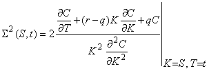 .
Equation 3
Given the market-observed prices of plain vanilla
options today, this equation determines the local volatility at time  if the stock
price is equal to
 . In any
arbitrage free model, the quantity on the right-hand side of this equation is
guaranteed to be positive [1], although in practice interpolation and/or
extrapolation effects will often lead to negative values of
 .
Furthermore, numerical effects for deep out-of-the-money
options, when both the numerator and denominator of Equation 3 tend to zero, lead to badly behaved local volatility
functions. For this reason, it is
preferable to rewrite the equation directly in terms of implied volatilities,
defined through the relationship with Black-Scholes option prices  :

Using this relationship to substitute for the derivatives
in Equation
3 gives [1], [18]
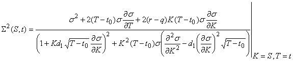 .
Equation 4
where:
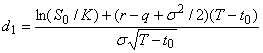 ,
and  and
 are respectively the
“market date”, on which the volatility smile is observed, and the underlying
price on that date.
Equation
4 is the basic result we use to generate the local
volatility function from the implied volatility surface.
The interpolation techniques used to compute the local
volatility function were originally discussed in the context of how to determine
the (risk-neutral) probability density function (pdf) of the underlying asset
from the volatility smile [5]. In addition
to the pricing functions described below, FINCAD provides a utility function to
back out the pdf from the smile along the same lines. A result originally due to Breeden and
Litzenberger [4] is that the pdf is proportional to the second
derivative of the option price with respect to the strike. If  is the current value
of the underlying, then the current value of a call option is:
 ,
where  is the (risk-neutral)
probability density function of the asset.
Differentiating twice with respect to gives:
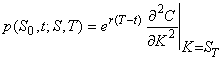 .
It again proves to be useful to write this in
terms of the implied volatility directly (see, e.g., [14]):
 ,
Equation 5
where
 is as above and
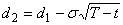 .
Given a market-observed smile, the FINCAD
function aaSmile_pdf
computes this pdf, and its first four moments (mean, variance, skew and
kurtosis).
The smoothing techniques discussed in [5] were applied to the smile to ensure that the
corresponding pdf is well-behaved, smooth and, in particular, everywhere
positive. Numerical effects for
non-smooth volatility smiles easily give rise to wildly oscillating, and
negative, values of the pdf.
Pricing Methodology
The suite of functions described in this document allow
the user to compute the price and risk statistics for plain vanilla options,
binary options (digital all-or-nothing calls or puts), a portfolio of plain
vanillas, a host of trading strategies (listed in the Appendix) and options
with arbitrary piecewise linear payoff functions.
The functions which deal solely with current valuation of
European options (aaOption_smile_eu_p and aaOption_smile_payoff_eu_p)
use only the closed form Black-Scholes formula.
The functions aaOption_LV_smile_p and aaOption_LV_smile_payoff_p,
on the other hand, use numerical finite-difference methods on the no-arbitrage
PDE (Equation
1) to compute the price and risk statistics of the options,
portfolios or strategies. These latter
two functions further allow for forward valuation (of both American and
European options). To forward value an
option, the valuation date d_v should be set to be greater than today’s “market
date” d_mkt, the date on which the implied volatility smile is observed. The underlying price should also be set to the
forward price (or expectation value) of the underlying asset, or any other
scenario value.
Current Valuation of European Options
To price European options today we need only interpolate
and/or extrapolate to the relevant strike prices from the market-observed
implied volatility smile. Except for
forward valuation, there is no need to consider the local volatility function,
since the interpolated implied volatilities can be substituted directly into
the Black-Scholes formula to obtain the option price and risk statistics. The functions aaOption_smile_eu_p
and aaOption_smile_payoff_eu_p
do the relevant interpolation and/or extrapolation, and then internally call aaBSG
or – in the case of a binary option – aaDigital_AON. The prices of a call () and put ( ) option are
 ,
 ,
and those of a Binary call ( ) and Binary put (
 ) option are
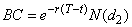 ,
 ,
where  is the cumulative
normal distribution. See the Black-Scholes Generalized
and the Binary
Options FINCAD Math Reference documents for further details of these
functions.
The function aaOption_smile_eu_tbl
exposes the results of the interpolation and/or extrapolation routines,
returning the interpolated implied volatility smile as discussed in the
Interpolation section below.
Note that the Greeks returned by these functions are the
Black-Scholes Greeks, which may not be what the user is most interested
in. One can instead bump the underlying
quantities and re-compute price either with the same smile (sticky-strike) or at
a shifted smile (stick-delta).
American and/or Forward Valuation of European Options
The FINCAD functions aaOption_LV_smile_p,
aaOption_LV_smile_payoff_p
all use finite difference methods on the no-arbitrage PDE (Equation 1). More
specifically, they use the Crank-Nicolson scheme which is unconditionally
stable (the von Neumann stability criterion is discussed in [1]) and has the best convergence properties as compared
to the fully implicit or fully explicit schemes. For a discussion of the general procedure
see, e.g., [18] and for an application to local volatility models,
see [1].
The first step is to set up a grid in which time runs from
the valuation date to the maturity date of the option, and we set the minimum
and maximum values of the underlying asset in such a way as to capture most of
the possible movements in the asset price.
As discussed in [1], it is possible to set the grid size such that the
(risk-neutral) probability of the underlying price at maturity falling outside
the grid is roughly 0.01%. To ensure
this, we take:
 ,
 .
Equation 6
with  is the average implied
volatility in the market-observed volatility smile. We further arrange the grid such that the
present price of the underlying asset lies exactly on a row of grid points.
The second step is to determine the values of the local
volatility function at each node of the grid, through Equation 4. We thus need
the values of the implied volatility and its derivatives on each grid point
(the derivatives can be had through a standard finite difference approximation along
the lines discussed in [16]). This is a
similar, though somewhat more involved, interpolation and extrapolation problem
to that discussed above, which we will discuss in the Interpolation section
below. The function aaOption_LV_smile_tbl
exposes the results of this interpolation procedure.
See the Option Pricing using a Local Volatility
Model FINCAD Math Reference document for further details of the
implementation of the Crank-Nicolson scheme.
Note that the Greeks returned by these functions are the
model implied Greeks (the finite difference approximations to the relevant
derivatives), which may not be what the user is most interested in. As above, one can instead bump the underlying
quantities and re-compute price either with the same smile (sticky-strike) or at
a shifted smile (stick-delta).
Interpolation
The local volatility function used in the numerical
pricing routines is given in terms of the implied volatility through Equation 4. To compute
the local volatility at any grid point, the values of both the implied
volatility and its derivatives must be known.
To deal with the derivatives, we use a simple finite difference
approximation, as in [16], so that only values of the implied volatility on
each grid point and its nearest neighbors need be computed. At any rate, some form of interpolation
procedure is necessary. There are
various techniques discussed in the literature, the topic being an area of
ongoing research (see, e.g., [9] and [16]).
Whichever method one uses, numerical effects often give
rise to quite badly-behaved local volatility functions. Small differences in the implied volatility
and, in particular, in its curvature in the strike dimension, lead to large spikes
in the local volatility function. In
addition to this, the value of can fairly easily
become negative. We deal with the latter
problem by cutting off the local volatility function at 2%. The former problem – the dependence on the
curvature of the implied volatility – can be reduced through a smoothing
routine, so that spikes in the derivatives do not propagate through to the
local volatility function so easily.
The smoothed cubic spline technique we use here was first
discussed in the context of implied (risk-neutral) probability density
functions [5], and applied to the implied volatility surface in [10]. For each
(fixed) value of option maturity which we are interested in, we apply a
smoothed cubic spline in the strike dimension.
The smoothing procedure, controlled by the smoothing_param input,
results in a cubic spline which no longer goes through all the data points
(strike vs. implied volatility) but has a smaller absolute value of the
curvature (in the strike direction).
Note that the volatility smile data can be entered in one
of three formats, as explained in the Description of
Inputs section. With the
exception of the function aaSmile_pdf, all interpolation is done in
strike space, so the smile_tbl input is internally converted into the strike
vs. implied volatility if need be.
The first step is to pick the data points from the smile
which the smoothed spline will be applied to.
The functions aaOption_smile_eu_p, aaOption_smile_payoff_p
and aaOption_smile_eu_tbl
need values of implied volatility at a single maturity only (the maturity of
the European option at hand), whereas the functions aaOption_LV_smile_p,
aaOption_LV_smile_payoff_p
and aaOption_LV_smile_tbl
need values of the implied volatility at every point in the grid which is set
up internally to price the options. In
particular, values at every time step between the valuation date d_v and the
option expiry date d_exp are needed.
Current Valuation of European Options
In this case, the user is most likely to have given values
of the implied volatility for options with that maturity (but varying strikes)
in the smile_tbl input. The data points
(strike vs. implied volatility) are then just those supplied explicitly by the
user. If data points for that maturity
are not in the smile_tbl input, however, then we perform an interpolation
and/or extrapolation in the maturity dimension to generate some representative
number of data points (strike vs. implied volatility) for the option maturity
in question.
In that case, depending on the interp_smile input, we
construct a bi-linear, bi-cubic or thin-plate spline through all points in the
smile_tbl, and out to the extreme values of the strikes and maturities which
are in that table. We then read off the
implied volatility values for some representative number of strike prices
between the two extremes. These are the
data points to which we apply the smoothing routine.
In either case, before applying the smoothing algorithm,
we add two extra points at constant values of volatility to both ends (small
strike, large strike) of the set of data points (strike vs. implied
volatility). This is to ensure that the
implied volatility smile is extrapolated to constant values. This has the effect of extrapolating the
corresponding (risk-neutral) probability density function to have lognormal
tails [3].
The smoothing routine is applied to this single set of
data points at a fixed option maturity.
American and/or Forward Valuation of European Options
As for the latter case above, we must first perform an
interpolation and/or extrapolation in the maturity dimension to generate some
representative number of data points, this time at each time step in the grid. This pre-smoothed function is again generated
in one of three ways, depending on the interp_smile input: either bi-linear,
bi-cubic or thin-plate splines are used.
The bi-linear and bi-cubic splines will only work well if a regular grid
of points in the smile_tbl is supplied.
For this reason, the thin-plate spline is preferable: this is the
natural generalization of the cubic spline to two dimensions, resulting in a
surface which goes through each point given by the user in the smile_tbl[4].
The interp_smile input also affects the extrapolation
method used. The bi-linear and bi-cubic
splines will extrapolate to constant values at the edges of the grid used in
the numerical routines. To force the
thin plate spline to extrapolate to constant values, however, we first add
points to the smile_tbl out to the edges of the grid, at constant values of the
implied volatility. The thin plate
spline is then constructed through the new, extrapolated table.
Note that the user can override this extrapolation
procedure by adding extra dummy points to the smile_tbl input. It is easy, for example, to force
extrapolation at a specific constant value of the implied volatility, or to
force some non-constant extrapolation by adding the necessary extra points.
Given this surface, at each maturity of interest, we read
off a representative number of values of the implied volatility between the minimum
and maximum ranges of the underlying price.
The smoothing routine is applied at each time step to this set of data
points.
Smoothing the Implied Volatility Surface
A smoothed cubic spline is constructed from the set of
(strike vs. implied volatility) data points, either for a single option
maturity, or at each time step in the internal grid.
For the data points  and for a smoothing
parameter
 , we compute the minimizer
 of the penalized sum
of squares:
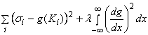
If the smoothing parameter  then the minimizer
is a standard cubic spline, the curve going through all data points. As
 is increased, the
curvature of the curve is reduced, and the curve will go through fewer data
points. In the limit
 , we obtain a least-squares fit. The minimizer is easily computed as a linear
algebra problem as described in, e.g., [11]. The result is
a function which is piecewise
continuous in its argument, .
It is difficult to give a general prescription for what
value of should be used
although, as a dimensionless number, values of the order of 10-2 to
0 seem to be sensible. One way to
determine a good choice is to check for a round trip on the implied volatility
data points using the function aaOption_LV_smile_p to get the prices of the
relevant European options, followed by aaBSG_iv to back
out the implied volatility corresponding to the numerical price. One often finds that  gives the best results
despite the badly-behaved local volatility function such a choice gives rise
to.
Armed with this smoothed cubic spline, for the European
functions, we read off the values of the implied volatility for the relevant
strikes, and substitute these into the Black-Scholes formula to give option
prices. To see the results of the
smoothing procedure, use the function aaOption_smile_eu_tbl,
which returns the smoothed implied volatility smile (the function above).
For the remaining functions, we read off the values of the
implied volatility for strike prices equal to the underlying prices in the
grid, and substitute these into (the finite difference version of) Equation 4. This gives
the values of the local volatility function at each grid point, used in the
Crank-Nicolson procedure described above.
To see both the resulting local volatility function and the smoothed
implied volatility surface, use the function aaOption_LV_smile_tbl,
which returns both surfaces. This allows
the results of using different values of the smoothing parameter to be
inspected.
Implied (Risk-Neutral) Probability Density Functions
As mentioned above, these smoothing techniques were
originally applied in the context of determining the pdf of an underlying asset
from the implied volatility smile [5]. The FINCAD
function aaSmile_pdf
allows the user to back out the pdf along those lines. To compute the pdf, we use Equation 5, which involves the values of the implied volatility
and its derivatives for a single option maturity, but for a range of strike
prices. The problem is essentially the
same as in the case of current valuation of European options discussed above.
In [5], however, the smoothing procedure was applied to the
implied volatility as a function of call option delta, rather than in strike
space as discussed above. The data
points were also weighted by the respective values of vega. Working in delta space was originally
considered by Malz [13], the idea being that out-of-the-money options would
then have less weight in the splining procedure. Working in delta space is also natural in the
FX world. The weighting by vega means
that these out-of-the-money data points have even less effect on the resulting
pdf[5]. (Actually, we use a dimensionless version of
vega as the weight, so that the smoothing parameter λ
remains dimensionless itself.)
At any rate, as for the non-forward valuation of European
options, we interpolate and/or extrapolate the data points in the smile_tbl
input to the relevant option maturity.
We also add points at constant values of implied volatility in the same
way, to ensure that the pdf has lognormal tails [3]. We smooth the
resulting set of data points in either strike space or in delta space,
depending on the interp_smile_pdf input.
If this switch is set to strike-space, then we compute the minimizer of:
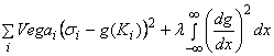 ,
which is the same as above, but with additional
weighting of the points by the options’ vega.
Since the asset price is unlikely to move beyond the values of  and
 in Equation 6,
we evaluate the smoothed spline at points between these values to determine the
pdf.
On the other hand, if the interp_smile_pdf switch is set
to delta-space we compute the minimizer of the above quantity, but in delta
space  is replaced by
 . The smile
data points (in strike space) are converted to data points in (call option)
delta space before the smoothing routine is applied. The resulting spline is evaluated at points
between 0 and
 (the maximum
possible range of call option
 ), to give the pdf as a function of , which is then converted back to strike space before
being returned to the user.
In either case, first four moments of the pdf are also
computed, allowing the mean, standard deviation, skew and kurtosis of the pdf
to be returned to the user. Define the
central moments  of a continuous
univariate pdf

 ,
where is the mean. The standard deviation is then just  ,and the skew and kurtosis are defined as:
skew =  , kurtosis
=
 .
With this definition, the kurtosis of the normal
distribution is equal to 3.
It is again difficult to give a general prescription for
what value of should be used
although, as above, it is a dimensionless number, so values of the order of 10-2
to 0 seem to be sensible. One should
plot the pdf output for different values, and also check the moments: the area,
for example, should be close to 1. invariably gives
a nonsensical pdf, oscillating between large positive and negative values. The user should increase until a sensible pdf
is obtained.
FINCAD Functions
aaOption_LV_smile_p
(price_u, payoff_type, strike_tbl, option_style, d_exp, d_v, d_mkt, smile_type,
smile_tbl, interp_smile, extrap_smile, smoothing_param, df_crv_std, df_crv_hld,
intrp, S_steps, t_steps, scheme, stat)
Calculates the price and risk statistics of a standard
option, a standard option strategy, or an option portfolio, from the implied
volatility smile. The function uses
local volatility in conjunction with finite difference methods on the
underlying no-arbitrage PDE, and handles European and American exercise
features as well as forward valuation.
aaOption_LV_smile_payoff_p
(price_u, payoff_tbl, option_style, d_exp, d_v, d_mkt, smile_type, smile_tbl,
interp_smile, extrap_smile, smoothing_param, df_crv_std, df_crv_hld, intrp,
S_steps, t_steps, scheme, stat)
Calculates the price and risk statistics of an option with
a freestyle payoff from the implied volatility smile. The function uses local volatility in
conjunction with finite difference methods on the underlying no-arbitrage PDE,
and handles European and American exercise features as well as forward
valuation.
aaOption_smile_eu_p
(price_u, payoff_type, strike_tbl, d_exp, d_v, smile_type, smile_tbl,
interp_smile, extrap_smile, smoothing_param, df_crv_std, df_crv_hld, intrp,
stat)
Calculates the price and risk statistics of a European
plain vanilla call or put option a standard European option strategy, or a
user-defined portfolio of European plain vanilla options, from the implied
volatility smile. The function
interpolates implied volatilities from the smile to use in the Black-Scholes
formula.
aaOption_smile_payoff_eu_p
(price_u, payoff_tbl, d_exp, d_v, smile_type, smile_tbl, interp_smile, extrap_smile,
smoothing_param, df_crv_std, df_crv_hld, intrp, stat)
Calculates the price and risk statistics of a European
option with a freestyle payoff from the implied volatility smile. The function interpolates implied
volatilities from the smile to use in the Black-Scholes formula.
aaOption_LV_smile_tbl
(price_u, d_exp, d_v, d_mkt, smile_type, smile_tbl, interp_smile, extrap_smile,
smoothing_param, df_crv_std, df_crv_hld, intrp, S_steps, t_steps, numerical
method, table_type)
Calculates a smooth implied volatility surface and a local
volatility function from a set of implied volatilities. This function can be used to expose the
results of the various interpolation routines used on the implied volatility
data, and the corresponding local volatility function used in numerical
solutions of the no-arbitrage PDE.
aaOption_smile_eu_tbl
(price_u, d_exp, d_v, smile_type, smile_tbl, interp_smile, extrap_smile, smoothing_param,
df_crv_std, df_crv_hld, intrp, K_tbl, table_type)
Calculates a smooth implied volatility smile from a set of
implied volatilities. This function can
be used to expose the results of the various interpolation routines used on the
implied volatility data when pricing European options from the smile.
aaSmile_pdf
(price_u, d_exp, d_mkt, smile_type, smile_tbl, interp_smile_pdf, extrap_smile, smoothing_param,
df_crv_std, df_crv_hld, intrp, K_S_tbl, table_type)
Calculates a smooth implied volatility smile, a (risk-neutral)
probability density function (PDF) of the underlying asset, and the mean,
standard deviation, skew and kurtosis of the PDF, from a set of implied
volatilities.
Description of Inputs
aaOption_LV_smile_p
|
Input Argument |
Type |
Description |
|
price_u |
number |
current value of the underlying stock |
|
payoff_type |
number |
switch to select the payoff of the option/strategy: 1. portfolio
(user-defined), 2. vanilla
call, 3. vanilla
put, 4. binary
call, 5. binary
put, 6. call
(bull) spread, 7. put
(bear) spread, 8. risk
reversal (collar), 9. seagull,
10. straddle,
11. strangle,
12. guts,
13. butterfly,
14. condor,
15. iron
butterfly, 16. iron
condor, 17. box,
18. ratio
call spread, 19. ratio
put spread, 20. synthetic
forward, 21. participating
forward (put), 22. participating
forward (call), 23. call
ladder, 24. put
ladder, 25. call
spread vs. put, 26. put
spread vs. call, 27. straddle
vs. call, 28. straddle
vs. put. The choice will affect the form of the
strike_tbl input. |
|
strike_tbl |
table or number |
table of (possibly time-varying) strikes to define the
option, portfolio or strategy; see below for details |
|
option_style |
number |
switch to select the option style (European,
American). If option_style = American
then all the options in the portfolio or strategy can be exercised
independently. |
|
d_exp |
date |
maturity date of the option |
|
d_v |
date |
valuation date |
|
d_mkt |
date |
market date on which the implied volatility smile is
observed |
|
smile_type |
number |
switch to select the type of smile_tbl given as an input |
|
smile_tbl |
table |
the market observed implied volatility smile |
|
interp_smile |
number |
switch to select the interpolation method to use on the
implied volatility smile |
|
extrap_smile |
number |
switch to select the extrapolation method to use on the
implied volatility smile (currently only constant extrapolation is available) |
|
smoothing_param |
table |
a table containing the smoothing parameter to use in the
interp_smile method |
|
df_crv_std |
table or rate |
risk-free discount factor curve. The discount factor curve may be input as
an N×2 table (column 1 = date, column 2 = discount factor), or as a single
cell containing a rate. If input as a single rate, there are three format choices:
1.
a rate (1×1 table); or 2.
a rate and a rate quotation basis as per
Switch 43 (1×2 table); or 3.
a rate, a rate quotation basis, and an accrual
method as per Switch 331 (1×3 table). If the basis or accrual methods are not
provided, they are assumed to be annual, actual/365. An N×2 flat-rate discount factor curve is
constructed internally between the value date and the expiry date, using the
rate, basis and accrual method. |
|
df_crv_hld |
table or rate |
dividend discount factor curve. The discount factor curve may be input as
an N×2 table (column 1 = date, column 2 = discount factor), or as a single
cell containing a rate. If input as a single rate, there are three format choices:
1.
a rate (1×1 table); or 2.
a rate and a rate quotation basis as per
Switch 43 (1×2 table); or 3.
a rate, a rate quotation basis, and an accrual
method as per Switch 331 (1×3 table). If the basis or accrual methods are not
provided, they are assumed to be annual, actual/365. An N×2 flat-rate discount factor curve is
constructed internally between the value date and the expiry date, using the
rate, basis and accrual method. |
|
intrp |
number |
switch to select which interpolation method to use on the
discount factor curves (linear, cubic spline, exponential, linear spot rates) |
|
S_steps |
number |
number of steps to use in the underlying (S) direction |
|
t_steps |
number |
number steps to use in the time (t) direction |
|
scheme |
table or number |
switch to select which numerical method to use to solve
the PDE (currently only Crank-Nicolson is implemented) |
|
stat |
table or number |
switch to select which output the user wants; see Description of Outputs section |
aaOption_LV_smile_payoff_p
|
Input Argument |
Type |
Description |
|
price_u |
number |
current value of the underlying stock |
|
payoff_tbl |
table |
table defining the payoff profile. This is an N×2 table (column 1 =
underlying, column 2 = payoff) specifying the payoff at various values of the
underlying. A piecewise linear payoff
function is constructed internally from this data, so it is important to
enter all the points necessary to construct the correct (piecewise linear)
payoff. |
|
option_style |
number |
as above |
|
d_exp |
date |
maturity date of the option |
|
d_v |
date |
valuation date |
|
d_mkt |
date |
market date on which the implied volatility smile is
observed |
|
smile_type |
number |
switch to select the type of smile_tbl given as an input |
|
smile_tbl |
table |
the market observed implied volatility smile |
|
interp_smile |
number |
switch to select the interpolation method to use on the
implied volatility smile |
|
extrap_smile |
number |
switch to select the extrapolation method to use on the
implied volatility smile (currently only constant extrapolation is available) |
|
smoothing_param |
table |
a table containing the smoothing parameter to use in the
interp_smile method |
|
df_crv_std |
table or rate |
as above |
|
df_crv_hld |
table or rate |
as above |
|
intrp |
number |
as above |
|
S_steps |
number |
number of steps to use in the underlying (S) direction |
|
t_steps |
number |
number steps to use in the time (t) direction |
|
scheme |
table or number |
switch to select which numerical method to use to solve
the PDE (currently only Crank-Nicolson is implemented) |
|
stat |
table or number |
switch to select which output the user wants; see Description of Outputs section |
aaOption_smile_eu_p
|
Input Argument |
Type |
Description |
|
price_u |
number |
current value of the underlying stock |
|
payoff_type |
number |
switch to select the payoff of the option/strategy: 1.
portfolio (user-defined), 2. vanilla
call, 3. vanilla
put, 4. binary
call, 5. binary
put, 6. call
(bull) spread, 7. put
(bear) spread, 8. risk
reversal (collar), 9. seagull,
10. straddle,
11. strangle,
12. guts,
13. butterfly,
14. condor,
15. iron
butterfly, 16. iron
condor, 17. box,
18. ratio
call spread, 19. ratio
put spread, 20. synthetic
forward, 21. participating
forward (put), 22. participating
forward (call), 23. call
ladder, 24. put
ladder, 25. call
spread vs. put, 26. put
spread vs. call, 27. straddle
vs. call, 28. straddle
vs. put. The choice will affect the form of the
strike_tbl input. |
|
strike_tbl |
table or number |
table of (possibly time-varying) strikes to define the
option, portfolio or strategy; see below for details |
|
d_exp |
date |
maturity date of the option |
|
d_v |
date |
valuation date |
|
smile_type |
number |
switch to select the type of smile_tbl given as an input |
|
smile_tbl |
table |
the market observed implied volatility smile |
|
interp_smile |
number |
switch to select the interpolation method to use on the
implied volatility smile |
|
extrap_smile |
number |
switch to select the extrapolation method to use on the
implied volatility smile (currently only constant extrapolation is available) |
|
smoothing_param |
table |
a table containing the smoothing parameter to use in the
interp_smile method |
|
df_crv_std |
table or rate |
as above |
|
df_crv_hld |
table or rate |
as above |
|
intrp |
number |
as above |
|
stat |
table or number |
switch to select which output the user wants; see Description of Outputs section |
aaOption_smile_payoff_eu_p
|
Input Argument |
Type |
Description |
|
price_u |
number |
current value of the underlying stock |
|
payoff_tbl |
number |
table defining the payoff profile. This is an N×2 table (column 1 = underlying,
column 2 = payoff) specifying the payoff at various values of the
underlying. A piecewise linear payoff
function is constructed internally from this data, so it is important to
enter all the points necessary to construct the correct (piecewise linear)
payoff. |
|
d_exp |
date |
maturity date of the option |
|
d_v |
date |
valuation date |
|
smile_type |
number |
switch to select the type of smile_tbl given as an input |
|
smile_tbl |
table |
the market observed implied volatility smile |
|
interp_smile |
number |
switch to select the interpolation method to use on the
implied volatility smile |
|
extrap_smile |
number |
switch to select the extrapolation method to use on the
implied volatility smile (currently only constant extrapolation is available) |
|
smoothing_param |
table |
a table containing the smoothing parameter to use in the
interp_smile method |
|
df_crv_std |
table or rate |
as above |
|
df_crv_hld |
table or rate |
as above |
|
intrp |
number |
as above |
|
stat |
table or number |
switch to select which output the user wants; see Description of Outputs section |
aaOption_LV_smile_tbl
|
Input Argument |
Type |
Description |
|
price_u |
number |
current value of the underlying stock |
|
d_exp |
date |
maturity date of the option |
|
d_v |
date |
valuation date |
|
d_mkt |
date |
market date on which the implied volatility smile is
observed |
|
smile_type |
number |
switch to select the type of smile_tbl given as an input |
|
smile_tbl |
table |
the market observed implied volatility smile |
|
interp_smile |
number |
switch to select the interpolation method to use on the
implied volatility smile |
|
extrap_smile |
number |
switch to select the extrapolation method to use on the
implied volatility smile (currently only constant extrapolation is available) |
|
smoothing_param |
table |
a table containing the smoothing parameter to use in the
interp_smile method |
|
df_crv_std |
table or rate |
as above |
|
df_crv_hld |
table or rate |
as above |
|
intrp |
number |
as above |
|
S_steps |
number |
number of steps to use in the underlying (S) direction |
|
t_steps |
number |
number steps to use in the time (t) direction |
|
table_type |
number |
switch to select which output the user wants; see Description of Outputs section |
aaOption_smile_eu_tbl
|
Input Argument |
Type |
Description |
|
price_u |
number |
current value of the underlying stock |
|
d_exp |
date |
maturity date of the option |
|
d_v |
date |
valuation date |
|
smile_type |
number |
switch to select the type of smile_tbl given as an input |
|
smile_tbl |
table |
the market observed implied volatility smile |
|
interp_smile |
number |
switch to select the interpolation method to use on the
implied volatility smile |
|
extrap_smile |
number |
switch to select the extrapolation method to use on the
implied volatility smile (currently only constant extrapolation is available) |
|
smoothing_param |
table |
a table containing the smoothing parameter to use in the
interp_smile method |
|
df_crv_std |
table or rate |
as above |
|
df_crv_hld |
table or rate |
as above |
|
intrp |
number |
as above |
|
K_tbl |
table |
table of strike prices for which to return the implied
volatility |
|
table_type |
table or number |
switch to select which output the user wants; see Description of Outputs section |
aaSmile_pdf
|
Input Argument |
Type |
Description |
|
price_u |
number |
current value of the underlying stock |
|
d_exp |
date |
maturity date of the option |
|
d_mkt |
date |
market date on which the implied volatility smile is
observed |
|
smile_type |
number |
switch to select the type of smile_tbl given as an input |
|
smile_tbl |
table |
the market observed implied volatility smile |
|
interp_smile_pdf |
number |
switch to select the interpolation method to use on the
implied volatility smile |
|
extrap_smile |
number |
switch to select the extrapolation method to use on the
implied volatility smile (currently only constant extrapolation is available) |
|
smoothing_param |
table |
a table containing the smoothing parameter to use in the
interp_smile method |
|
df_crv_std |
table or rate |
as above |
|
df_crv_hld |
table or rate |
as above |
|
intrp |
number |
as above |
|
K_S_tbl |
table |
table of underlying values for which to return the (risk-neutral)
probability density function |
|
table_type |
table or number |
switch to select which output the user wants; see Description of Outputs section |
smile_tbl
In more detail, the implied volatility smile in all of the
above functions can be specified in one of three ways (in all cases, the option
maturities must be given as dates > d_mkt, or as number of years since d_mkt):
·
if smile_type = strike
vs. implied volatility
smile_tbl
|
maturity |
exercise price |
implied volatility |
|
|
|
|
|
… |
… |
… |
|
|
|
|
|
|
|
|
|
… |
… |
… |
|
|
|
|
|
… |
… |
… |
|
|
|
|
|
… |
… |
… |
|
|
|
|


where the  are
implied (Black-Scholes) volatilities, as a function of strikes
 and maturities
 .
·
if smile_type = delta
vs. implied volatility
smile_tbl
|
maturity |
delta |
implied volatility |
|
|
|
|
|
… |
… |
… |
|
|
|
|
|
|
|
|
|
… |
… |
… |
|
|
|
|
|
… |
… |
… |
|
|
|
|
|
… |
… |
… |
|
|
|
|


where now the volatilities are entered as a function
of deltas  and maturities
 . Since
 for a put and
 for a call, the user
can enter either call or put deltas (or a mixture), without having to specify
which is which.
·
if smile_type = strike
vs. price
smile_tbl
|
maturity |
strike |
call/put |
price |
|
|
|
1/2 |
|
|
… |
… |
… |
… |
|
|
|
1/2 |
|
|
|
|
1/2 |
|
|
… |
… |
… |
… |
|
|
|
1/2 |
|
|
… |
… |
… |
… |
|
|
|
1/2 |
|
|
… |
… |
… |
… |
|
|
|
1/2 |
|


where the  are
the prices of plain vanilla European options, either calls (1) or puts (2).
strike_tbl
The various options/portfolios/strategies in the functions
aaOption_LV_smile_p
and aaOption_smile_eu_p
are specified through the payoff_type and strike_tbl inputs. The various strategies FINCAD supports are
all described in [12], where P&L diagrams can also be found; see the
Appendix for a breakdown into their constituent plain vanillas. The strike_tbl should specify the relevant
exercise prices, and must take one of the following forms.
·
if payoff_type = portfolio
(user-defined), the details of the options in the portfolio must be
specified.
strike_tbl
|
long/short |
call/put |
strike |
|
|
1/2 |
|
|
|
1/2 |
|
|
… |
… |
… |
|
|
1/2 |
|


Here,  denotes respectively a
long/short position in
 options, which are
either calls (1) or puts (2), with the given strikes. The individual options must be either all
European or all American.
·
if payoff_type = vanilla
call, vanilla put, straddle or synthetic forward, only a single exercise
price must be entered.
strike_tbl
|
exercise price |
|
|
·
if payoff_type = vanilla
call or vanilla put (and if option_style = American), a time-varying
exercise price can also be specified.
strike_tbl
|
effective date |
terminating date |
exercise price |
|
|
|
|
|
|
|
|
|
… |
… |
… |
|
|
|
|


where
each terminating date must be greater than the
corresponding effective date  and
each effective date must be greater than or equal to
the previous terminating date 
By allowing for gaps in this table, blackout periods
are thus allowed (alternatively, a blackout period can be specified by setting  ).
·
if payoff_type = binary
call or binary put, a single exercise price and a cash payout must be
specified.
strike_tbl
|
exercise price |
cash payout |
|
|
|
The binaries are digital all-or-nothing options,
which pay a fixed amount of cash (and can be European or American).
·
if payoff_type = participating
forward (put) or participating forward (call), a single exercise price
and a percentage (the degree of participation) must be specified.
strike_tbl
|
exercise price |
percentage |
|
|
|

·
if payoff_type = straddle
vs. call or straddle vs. put, then two distinct exercise prices must be
specified.
strike_tbl
|
exercise price 1 |
exercise price 2 |
|
|
|
·
if payoff_type = call
(bull) spread, put (bear) spread, risk reversal (collar), strangle, guts,
butterfly, condor, box, then two distinct exercise prices must be
specified.
strike_tbl
|
exercise price 1 |
exercise price 2 |
|
|
|
where the restriction  applies.
·
if payoff_type = call
spread vs. put or put spread vs. call, then three distinct exercise
prices must be specified.
strike_tbl
|
exercise price 1 |
exercise price 2 |
exercise price 3 |
|
|
|
|
where the restriction applies.
·
if payoff_type = seagull,
iron butterfly, call ladder, put ladder, then three distinct exercise
prices must be specified.
strike_tbl
|
exercise price 1 |
exercise price 2 |
exercise price 3 |
|
|
|
|
where the restriction  applies.
·
if payoff_type = ratio
call spread or ratio put spread, then two exercise prices and two
integers must be specified (the integers give the ratio of the spread).
strike_tbl
|
exercise price 1 |
exercise price 2 |
number 1 |
number 2 |
|
|
|
|
|


where the restrictions  and
 apply.
·
if payoff_type = iron
condor then four distinct exercise prices must be specified.
strike_tbl
|
strike 1 |
strike 2 |
strike 3 |
strike 4 |
|
|
|
|
|


where the restriction  applies.
payoff_tbl
The functions aaOption_LV_smile_payoff_p
and aaOption_smile_payoff_eu_p
allow the user to specify an arbitrary (piecewise linear) payoff function. This is done through the payoff_tbl input
which must take the following form:
payoff_tbl
|
underlying |
payoff |
|
|
|
|
|
|
|
… |
… |
|
|
|


where the payoff  is given for a set of
underlying values
 . A piecewise linear
payoff function is constructed from this data internally, so it is important
that the user enter enough points to construct the payoff of interest. Outside of the range of given underlying
values, the payoff is constructed by linear extrapolation from the last two (or
first two) points in the payoff_tbl.
Description of Outputs
aaOption_LV_smile_p, aaOption_LV_smile_payoff_p
These functions output the price and risk statistics
of the relevant option, strategy or portfolio.
There is one additional output, which is the minimum suggested number of
steps in the underlying direction; this is discussed in the Finite Difference section above.
|
Output Statistics |
Type |
Description |
|
fair value |
number |
fair value of the option. |
|
delta |
number |
rate of change in the fair value of the option per change
in the current value of the underlying stock.
This is the derivative of the option price with respect to the current
value of the underlying. |
|
gamma |
number |
rate of change in the value of delta per change in the
current value of the underlying stock.
This is the second derivative of the option price with respect to the
current value of the underlying. |
|
theta |
number |
rate of change in the fair value of the option per one day
decrease in the option time. This is
the negative of the derivative of the option price with respect to the option
time (in years), divided by 365. |
|
vega |
number |
change in the fair value of the option per 1% change in
annual volatility. |
|
rho of rate |
number |
change in the fair value of the option per 1% change in
the risk-free rate. |
|
rho of holding cost |
number |
change in the fair value of the option per 1% change in
the dividend rate. |
|
minimum S_steps |
number |
the minimum suggested number of S_steps |
aaOption_smile_eu_p, aaOption_smile_payoff_eu_p
These functions output the price and risk statistics
of the relevant option, strategy or portfolio.
|
Output Statistics |
Type |
Description |
|
fair value |
number |
fair value of the option. |
|
delta |
number |
rate of change in the fair value of the option per change
in the current value of the underlying stock.
This is the derivative of the option price with respect to the current
value of the underlying. |
|
gamma |
number |
rate of change in the value of delta per change in the
current value of the underlying stock.
This is the second derivative of the option price with respect to the
current value of the underlying. |
|
theta |
number |
rate of change in the fair value of the option per one day
decrease in the option time. This is
the negative of the derivative of the option price with respect to the option
time (in years), divided by 365. |
|
vega |
number |
change in the fair value of the option per 1% change in
annual volatility. |
|
rho of rate |
number |
change in the fair value of the option per 1% change in
the risk-free rate. |
|
rho of holding cost |
number |
change in the fair value of the option per 1% change in
the dividend rate. |
aaOption_LV_smile_tbl
This function will output a table of either implied
volatilities or local volatilities at each point in the grid used to solve the
no-arbitrage PDE (Equation
1). It thus
allows the user to examine the results of the smoothing algorithm used on the
implied volatility surface, and also to examine the local volatility function
used in the finite-difference pricing algorithm. Since the grid is set up internally, there is
no need for the user to specify at which points to return the values of the
volatilities:
·
if table_type = implied
volatility surface, then the values of the implied volatility surface (after
the smoothing algorithm) are returned at the points  and
 , where
 and are the grid points
set as explained above.
output_tbl
|
maturity |
exercise price |
implied volatility |
|
|
|
|
|
… |
… |
… |
|
|
|
|
|
|
|
|
|
… |
… |
… |
|
|
|
|
|
… |
… |
… |
|
|
|
|
|
… |
… |
… |
|
|
|
|

The maturities  will be given
as number of years since d_v.
·
if table_type = local
volatility function, then the values of the local volatility function
(computed through Equation
4) are returned at the points and , the grid points set as explained above.
output_tbl
|
time |
underlying price |
local volatility |
|
|
|
|
|
… |
… |
… |
|
|
|
|
|
|
|
|
|
… |
… |
… |
|
|
|
|
|
… |
… |
… |
|
|
|
|
|
… |
… |
… |
|
|
|
|


The values  of time will be
given as number of years since d_v. The
local volatility output can thus be used as an input to the functions aaOption_LVtbl_p,
aaOption_LVtbl_payoff_p
and aaOption_LVtbl_iv,
for example to examine the forward dynamics of the implied volatility smile.
aaOption_smile_eu_tbl
This function will output a table of implied volatilities
at values of the strike price given through the K_tbl input. It thus allows the user to examine the
results of the smoothing algorithm used on the implied volatility surface in
the functions aaOption_smile_eu_p
and aaOption_smile_payoff_eu_p.
·
if table_type = implied
volatility smile, then the values of the implied volatility smile (after
the smoothing algorithm) are returned at the points  , as given in the K_tbl input.
K_tbl
|
exercise price |
|
|
|
|
|
… |
|
|

output_tbl
|
exercise price |
implied volatility |
|
|
|
|
|
|
|
… |
… |
|
|
|


aaSmile_pdf
This function will output a table either of implied
volatilities at values of the strike price given through the K_S_tbl input, or
of probabilities at values of the underlying price given through the K_S_tbl
input.
·
if table_type = implied
volatility smile, then the values of the implied volatility smile (after
the smoothing algorithm) are returned at the points  , as given in the K_S_tbl input.
K_S_tbl
|
exercise price |
|
|
|
|
|
… |
|
|
output_tbl
|
exercise price |
implied volatility |
|
|
|
|
|
|
|
… |
… |
|
|
|

·
if table_type = (risk-neutral)
probability density function, then the values
of the pdf are returned at the points  , as given through the K_S_tbl input. There are two different ways to determine
these points.
If interp_smile_pdf = delta-space
then the K_S_tbl should contain a single integer, the number of underlying
prices for which to return the pdf. The
values are determined internally, since the smoothing is done in delta-space.
K_S_tbl
|
number of points |
|
10 |
output_tbl
|
underlying price |
probability |
|
|
|
|
|
|
|
… |
… |
|
|
|


If interp_smile_pdf = strike-space
then the K_S_tbl should contain the values of the underlying prices for which to
return the pdf.
K_S_tbl
|
underlying price |
|
|
|
|
|
… |
|
|
output_tbl
|
underlying price |
probability |
|
|
|
|
|
|
|
… |
… |
|
|
|
·
if table_type = moments
of (risk-neutral) probability density function, then the values of the mean,
standard deviation, skew and kurtosis of the pdf are returned (the K_S_tbl
input is ignored in this case).
output_tbl
|
mean |
standard deviation |
skew |
kurtosis |
|
|
|
|
|


For badly-behaved pdfs, numerical effects may cause the
variance to be negative, in which case values of -1 are returned for the
standard deviation, the skew and the kurtosis.
The smoothing_param should be changed to get better results.
Examples
Example 1: American Call from the
Smile
Today is January 1, 2007.
Consider an at-the-money American call option that matures 6 months from
today. It has an exercise price of $50
for the life of the option. The
risk-free rate is 7.5% (annual compounding, actual/365 accrual), and the
dividend rate is 2.5% (annual compounding, actual/365 accrual).
Suppose we want to value the option “from the smile” as
observed today. To value a 6 month
option, we need implied volatilities for options with maturities up to and
including 6 months. The market data we
observe are as follows (implied volatilities of 3-month and 6-month options for
various strikes).
t_2033_1 – smile_tbl
|
maturity |
exercise price |
implied volatility |
|
1-Apr-2007 |
35 |
28% |
|
1-Apr-2007 |
40 |
26% |
|
1-Apr-2007 |
45 |
24% |
|
1-Apr-2007 |
50 |
23% |
|
1-Apr-2007 |
55 |
22% |
|
1-Apr-2007 |
60 |
21.5% |
|
1-Jul-2007 |
35 |
26.5% |
|
1-Jul-2007 |
40 |
26% |
|
1-Jul-2007 |
45 |
25.5% |
|
1-Jul-2007 |
50 |
25.1% |
|
1-Jul-2007 |
55 |
24.7% |
|
1-Jul-2007 |
60 |
24.4% |
We call the function aaOption_LV_smile_p
with the following inputs.
aaOption_LV_smile_p
|
Argument |
Description |
Example Data |
Switch |
Comments |
|
price_u |
underlying price |
50 |
|
|
|
payoff_type |
payoff |
2 |
vanilla call |
|
|
strike_tbl |
strike table |
50 |
|
a single strike to define the call |
|
option_style |
style of option |
2 |
American |
|
|
d_exp |
expiry date |
1-Jul-2007 |
|
6 months from today |
|
d_v |
value date |
1-Jan-2007 |
|
|
|
d_mkt |
date on which the smile is observed |
1-Jan-2007 |
|
no forward valuation |
|
smile_type |
type of smile table |
1 |
strike vs. implied volatility |
|
|
smile_tbl |
smile table |
t_2033_1 as above |
|
|
|
interp_smile |
interpolation method for the smile |
3 |
thin-plate (plus smoothing) |
|
|
extrap_smile |
extrapolation method for the smile |
1 |
constant extrapolation |
must = 1 |
|
smoothing_param |
smile interpolation parameters |
0 |
|
no smoothing |
|
df_crv_std |
discount factor curve – risk free |
7.5% |
|
annual compounding and actual/365 accrual is assumed |
|
df_crv_hld |
discount factor curve – holding cost |
2.5% |
|
annual compounding and actual/365 accrual is assumed |
|
intrp |
interpolation |
3 |
exponential |
not used for constant rates |
|
S_steps |
number of underlying steps |
200 |
|
|
|
t_steps |
number of time steps |
200 |
|
|
|
scheme |
numerical method |
1 |
Crank-Nicolson |
|
|
stat |
list of statistics |
1…8 |
|
|
With these inputs, the results are:
Results
|
Output Statistics |
Description |
Value |
|
1 |
fair value |
4.041994070 |
|
2 |
delta |
0.555501496 |
|
3 |
gamma |
0.045473112 |
|
4 |
theta |
-0.011064444 |
|
5 |
vega |
0.135446133 |
|
6 |
rho of rate |
0.115261111 |
|
7 |
rho of holding cost |
-0.137951067 |
|
8 |
minimum S_steps |
200 |
Since the minimum suggested number of S_steps is
200, we know that the inputs are such that we need less than 200 S_steps to
avoid any unstable numerical results; however, a minimum of 200 steps is always
recommended.
We can vary the interp_smile and the smoothing_param
inputs to see how dependent the option price and risk statistics are on the
interpolation procedure used on the implied volatility surface. We can also inspect the results of this
interpolation – both the interpolated implied volatility surface and the
resulting local volatility function by calling the function aaOption_LV_smile_tbl
with the following inputs:
aaOption_LV_smile_tbl
|
Argument |
Description |
Example Data |
Switch |
Comments |
|
price_u |
underlying price |
50 |
|
|
|
d_exp |
expiry date |
1-Jul-2007 |
vanilla call |
6 months from today |
|
d_v |
value date |
1-Jan-2007 |
|
|
|
d_mkt |
date on which the smile is observed |
1-Jan-2007 |
|
no forward valuation |
|
smile_type |
type of smile table |
1 |
strike vs. implied volatility |
|
|
smile_tbl |
smile table |
t_2033_1 as above |
|
|
|
interp_smile |
interpolation method for the smile |
3 |
thin-plate (plus smoothing) |
|
|
|
|
|
|
|
|
smoothing_param |
smile interpolation parameters |
0 |
|
no smoothing |
|
df_crv_std |
discount factor curve – risk free |
7.5% |
|
annual compounding and actual/365 accrual is assumed |
|
df_crv_hld |
discount factor curve – holding cost |
2.5% |
|
annual compounding and actual/365 accrual is assumed |
|
intrp |
interpolation |
3 |
exponential |
not used for constant rates |
|
S_steps |
number of underlying steps |
100 |
|
fewer steps for more manageable output |
|
t_steps |
number of time steps |
100 |
|
fewer steps for more manageable output |
|
table_type |
output table type |
2 |
local volatility surface |
|
The output is a large table, of local volatility
values on each grid point, which is most easily visualized through a pivot
table plot:
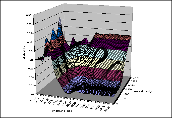
Figure 1
Example 2: European Butterfly from
the Smile
Today is January 1, 2007.
Consider a European butterfly option that matures 3 months from
today. It is built from two long calls
with exercise prices of $20 and $30, and two short calls with exercise prices
of $25. The current underlying price is
$25, the risk-free rate is 7.5% (annual compounding, actual/365 accrual), and
the dividend rate is 2.5% (annual compounding, actual/365 accrual).
Suppose we want to value the option “from the smile” as
observed today. To value a 3 month
option, we need implied volatilities for options with maturities up to and
including 3 months.
t_2033_2 – smile_tbl
|
maturity |
exercise price |
implied volatility |
|
1-Apr-2007 |
10 |
27% |
|
1-Apr-2007 |
15 |
26% |
|
1-Apr-2007 |
20 |
25.5% |
|
1-Apr-2007 |
25 |
25% |
|
1-Apr-2007 |
30 |
25.2% |
|
1-Apr-2007 |
35 |
25.5% |
|
1-Apr-2007 |
40 |
25.8% |
Since the strategy is built from European options,
the quickest, and most accurate valuation is to use the function aaOption_smile_eu_p
with the following inputs:
aaOption_smile_eu_p
|
Argument |
Description |
Example Data |
Switch |
Comments |
|
price_u |
underlying price |
25 |
|
|
|
payoff_type |
type of payoff |
13 |
butterfly |
|
|
strike_tbl |
strike table |
see below |
|
two strikes are needed to define the butterfly |
|
d_exp |
expiry date |
1-Apr-2007 |
|
3 months from today |
|
d_v |
value date |
1-Jan-2007 |
|
|
|
smile_type |
type of smile table |
1 |
strike vs. implied volatility |
|
|
smile_tbl |
smile table |
t_2033_2 as above |
|
|
|
interp_smile |
interpolation method for the smile |
3 |
thin-plate (plus smoothing) |
won’t have any effect here, since options with 3 month
maturities are given in t_2033_1 |
|
extrap_smile |
extrapolation method for the smile |
1 |
constant extrapolation |
must = 1 |
|
smoothing_param |
smile interpolation parameters |
0.001 |
|
|
|
df_crv_std |
discount factor curve – risk free |
7.5% |
|
annual compounding and actual/365 accrual is assumed |
|
df_crv_hld |
discount factor curve – holding cost |
2.5% |
|
annual compounding and actual/365 accrual is assumed |
|
intrp |
interpolation method |
3 |
exponential |
not used for constant rates |
|
stat |
list of statistics |
1…7 |
|
|
To specify the payoff of the strategy, we need two
exercise prices (those of the long calls) in the strike_tbl.
strike table
|
exercise price 1 |
exercise price 2 |
|
20 |
30 |
With these inputs, the results are:
Results
|
Output Statistics |
Description |
Value |
|
1 |
fair value |
2.614902875 |
|
2 |
delta |
-0.054882553 |
|
3 |
gamma |
-0.177298644 |
|
4 |
theta |
0.010201452 |
|
5 |
vega |
-0.068370960 |
|
6 |
rho of rate |
-0.008506978 |
|
7 |
rho of holding cost |
0.003220151 |
We can vary the interp_smile and the
smoothing_param inputs to see how dependent the option price and risk
statistics are on the interpolation procedure used on the implied volatility
surface. We can also inspect the results
of this interpolation by calling the function aaOption_smile_eu_tbl
with the following inputs:
aaOption_smile_eu_tbl
|
Argument |
Description |
Example Data |
Switch |
Comments |
|
price_u |
underlying price |
25 |
|
|
|
d_exp |
expiry date |
1-Apr-2007 |
|
3 months from today |
|
d_v |
value date |
1-Jan-2007 |
|
|
|
smile_type |
type of smile table |
1 |
strike vs. implied volatility |
|
|
smile_tbl |
smile table |
t_2033_2 as above |
|
|
|
interp_smile |
interpolation method for the smile |
3 |
thin-plate (plus smoothing) |
won’t have any effect here, since options with 3 month
maturities are given in t_2033_1 |
|
extrap_smile |
extrapolation method for the smile |
1 |
constant extrapolation |
must = 1 |
|
smoothing_param |
smile interpolation parameters |
0.001 |
|
|
|
df_crv_std |
discount factor curve – risk free |
7.5% |
|
annual compounding and actual/365 accrual is assumed |
|
df_crv_hld |
discount factor curve – holding cost |
2.5% |
|
annual compounding and actual/365 accrual is assumed |
|
intrp |
interpolation method |
3 |
exponential |
not used for constant rates |
|
K_tbl |
exercise prices |
see below |
|
|
|
table_type |
output table type |
1 |
implied volatility smile |
must be = 1 |
The K_tbl input contains the strike prices for which
to return the implied volatilities. Let
us assume that this takes the following form:
t_2035_1 – K_tbl
|
exercise price |
|
5 |
|
10 |
|
15 |
|
20 |
|
25 |
|
30 |
|
35 |
|
40 |
|
50 |
With these inputs, the output is a table of implied
volatilities for the above strike prices:
|
exercise price |
implied volatility |
|
5 |
27.035% |
|
10 |
26.821% |
|
15 |
26.114% |
|
20 |
25.460% |
|
25 |
25.092% |
|
30 |
25.184% |
|
35 |
25.492% |
|
40 |
25.749% |
|
50 |
25.807% |
Due to the smoothing routine, the returned values are
not the same as the input ones; the smoothed cubic spline does not go through
all the data points. One can vary the
smoothing parameter (or set it equal to zero to use a standard cubic spline),
and plot the results of this function to see the effects.
Example 3: Implied (Risk-Neutral) Probability Density Function from the
Smile
Suppose we are further interested in what is the (risk-neutral)
probability density function, 3 months from today, of the underlying asset in
the above example. That is, we want to
know what the pdf is which corresponds to the implied volatility smile given by
t_2033_2 above.
To compute the pdf, call the function aaSmile_pdf
with the following inputs:
aaSmile_pdf
|
Argument |
Description |
Example Data |
Switch |
Comments |
|
price_u |
underlying price |
25 |
|
|
|
d_exp |
expiry date |
1-Apr-2007 |
|
3 months from today |
|
d_v |
value date |
1-Jan-2007 |
|
|
|
smile_type |
type of smile table |
1 |
strike vs. implied volatility |
|
|
smile_tbl |
smile table |
t_2033_2 as above |
|
|
|
interp_smile_pdf |
space in which to interpolate the smile |
1 |
strike-space |
smooth in strike space rather than delta space |
|
extrap_smile |
extrapolation method for the smile |
1 |
constant extrapolation |
must = 1 |
|
smoothing_param |
smile interpolation parameters |
0.0001 |
|
|
|
df_crv_std |
discount factor curve – risk free |
7.5% |
|
annual compounding and actual/365 accrual is assumed |
|
df_crv_hld |
discount factor curve – holding cost |
2.5% |
|
annual compounding and actual/365 accrual is assumed |
|
intrp |
interpolation method |
3 |
exponential |
not used for constant rates |
|
K_S_tbl |
exercise prices |
see below |
|
|
|
table_type |
output table type |
2 |
(risk-neutral) probability density function |
|
The K_S_tbl input contains the underlying prices
for which to return the pdf. Instead of
reproducing this here, let us simply assume that this includes 100 points
between 15 and 40, in steps of 0.25 (underlying price = 15, 15.25, 15.5, …
39.5, 39.75, 40). The output is a table
of probabilities, which is most easily visualized through a scatter plot:
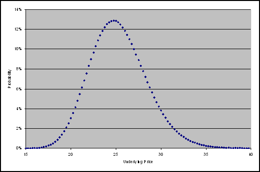
Figure 2
Different values of the smoothing_param should be
used to see the effects on the pdf. In
this case, the specific value does not make much of a difference, and indeed a
value of 0 gives a sensible pdf. One
could also choose to smooth in delta space rather than strike space. One should also check the implied volatility
smile output to see what the interpolated smile looks like with the given
smoothing parameter. Changing the
table_type input to implied volatility smile gives an output table of
interpolated implied volatilities which again are most easily visualized through
a scatter plot:
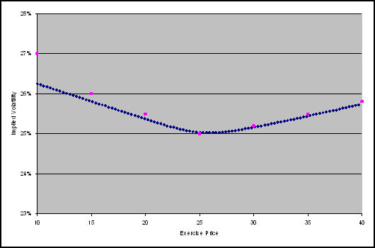
Figure 3
At any rate, with the above inputs, but with
table_type = 3 (moments of (risk-neutral) probability density function), we get
the following results for the moments of the above pdf.
Results
|
mean |
standard deviation |
skew |
kurtosis |
|
25.29532832 |
3.167647157 |
0.379388738 |
3.335389199 |
Related Functions
Calculates the price
and risk statistics of a standard option, a standard option strategy, or an
option portfolio, for a parameterized local volatility function such as those
which define the lognormal, normal, CEV and shifted lognormal stochastic
processes. The function uses finite
difference methods on the underlying no-arbitrage PDE, and handles European and
American exercise features.
Calculates the price
and risk statistics of a standard option, a standard option strategy, or an
option portfolio, given a user-defined local volatility function. The function uses finite difference methods
on the underlying no-arbitrage PDE, and handles European and American exercise
features.
Calculates the price
and risk statistics of an option with a freestyle payoff, for a parameterized
local volatility function such as those which define the lognormal, normal, CEV
and shifted lognormal stochastic processes.
The function uses finite difference methods on the underlying
no-arbitrage PDE, and handles European and American exercise features.
Calculates the price
and risk statistics of an option with a freestyle payoff, given a user-defined local
volatility function. The function uses
finite difference methods on the underlying no-arbitrage PDE, and handles European
and American exercise features.
Calculates the price
and risk statistics of a European plain vanilla call or put option, a standard
European option strategy, or a user-defined portfolio of European plain vanilla
options, for a parameterized local volatility function such as those which
define the lognormal, normal, CEV and shifted lognormal stochastic
processes. The function uses closed-form
solutions for standard processes.
Calculates the implied
volatility smile, for a parameterized local volatility function such as those
which define the lognormal, normal, CEV and shifted lognormal stochastic
processes. The function uses closed-form
solutions for standard processes.
Calculates the implied
volatility smile, given a user-defined local volatility function. The function uses finite difference methods
on the underlying no-arbitrage PDE.
Calculates the fair
value and risk statistics for European style options on securities with
continuous dividend yields.
Calculates the fair
value and risk statistics for a path independent digital all-or-nothing option.
Calculates the fair
value and risk measures for an American style option where the underlying pays
a continuous dividend. Based on the Cox
Rubinstein binomial model, the function can be used for options on spot foreign
exchange or equity indexes.
Appendix A: Trading Strategies
For further details
on these strategies, and for the relevant P&L diagrams, see [12].
The call (bull) spread is a long call with exercise price and a short call with
exercise price .
The put (bear) spread is a short put with exercise price and a long put with
exercise price .
The risk
reversal (collar) is a long put with exercise price and a short
call with exercise price .
The seagull is a short put with exercise price , a long put with exercise price  and a short call with exercise price
 .
The straddle
is a long call and a long put, both with exercise price .
The strangle is a long put with exercise price and a long call
with exercise price .
The guts is a long call with exercise price and a long put
with exercise price .
The butterfly is a long call (or put) with exercise price , a long call (or put) with exercise price and two short
calls (or puts) with exercise price
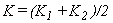 (midway between
and ). We assume
that the American butterfly consists of calls rather than puts.
The condor
is a long call (or put) with exercise
price , a long call (or put) with exercise price , a short call (or put) with exercise price  and a short
call (or put) with exercise price
 (so that the exercise
prices of the two short options are equally spaced between and ) . We assume
that the American condor consists of calls rather than puts.
The iron butterfly is a long straddle and a short strangle: a
short put with exercise price , a long call and a long put with exercise price and a short call with exercise price  .
The iron condor is a long strangle and a short strangle: a
short put with exercise price , a long put with exercise price , a long call
with exercise price and a short call with exercise price  .
The box
is a long call and a short put with exercise
price , and a long put and a short call with exercise price .
The ratio call spread is  short calls with exercise price and
 long calls with exercise price .
The ratio put spread is long puts with exercise price and short puts with exercise price .
The synthetic
forward is a long call and a short put, both with exercise price .
The participating
forward (put) is a long call and some percentage ( ) of a short put, both with exercise price .
The participating
forward (call) is a long put and some percentage () of a short call, both with exercise price .
The call ladder is a long call with exercise price , a short call with exercise price and a short call with exercise price  .
The put ladder is a short put with exercise price , a short put with exercise price and a long put with exercise price .
The call spread vs. put
is a long call with exercise price , a short call with exercise price and a short put with strike (usually, but not
always  ).
The put spread vs. call is a short put with exercise price , a long put with exercise price and a short call with exercise price (usually, but not always  ).
The straddle vs. call is a long call and a long put with exercise
price , and a short call with exercise price (usually, but not
always  ).
The straddle vs. put is a long call and a long put with exercise
price , and a short put with exercise price (usually, but not
always ).
References
[5]
Clews, R., Panigirtzoglou, N. and Proudman, J.
(2000) ‘Recent Developments in Extracting Information from Options Markets’, Bank of
Bliss, R. R. and Panigirtzoglou, N. (2000) ‘Testing the stability of implied
probability density functions’, Bank of England
Working Paper No 114. Available
on the Internet at http://www.bankofengland.co.uk/publications/workingpapers/wpabst00.htm#wp00.
[6]
Derman, E. and Kani,
[7]
Duffy, D. J. (2004), Financial
Instrument Pricing Using C++,
[8]
Dupire, B. (1994) ‘Pricing with a smile’, RISK, 7 (1), 18-20.
[9]
Fengler, M. R. (2005) Semiparametric Modeling of Implied Volatility,
[10]
Fengler, M. R. (2005) ‘Arbitrage-Free Smoothing
of the Implied Volatility Surface’, Humboldt-Universität
zu
[11]
Green, P. J. and Silverman, B. W. (1994) Nonparametric Regression and Generalized Linear Models,
[12]
LIFFE Management and Administration (2002), LIFFE Options: a guide to trading strategies. Available on the Internet at http://www.euronext.com/file/view/0,4245,1626_53424_516478967,00.pdf
[14]
Merton, R. (1973) ‘Theory of Rational Option
Pricing’,
[15] Press,
W. H., Teukolsky, S. A., Vetterling, W. T. and Flannery, B. P. (2002) Numerical Recipes in C++: The Art of Scientific Computing,
Cambridge: Cambridge University Press.
[16]
Rebonato, R. (2004) Volatility
and Correlation: the Perfect Hedger and the Fox, 2nd ed.,
[17]
Rubenstein, M. (1994) ‘Implied Binomial Trees’, Journal of Finance, 49 (3), 771-818.
[18]
Wilmott, P. (2006) Paul
Wilmott on Quantitative Finance, 2nd ed.,
Disclaimer
With respect to this document,
FinancialCAD Corporation (“FINCAD”) makes no warranty either express or
implied, including, but not limited to, any implied warranty of merchantability
or fitness for a particular purpose. In no event shall FINCAD be liable to
anyone for special, collateral, incidental, or consequential damages in
connection with or arising out of the use of this document or the information
contained in it. This document should not be relied on as a substitute for your
own independent research or the advice of your professional financial,
accounting or other advisors.
This information is subject to change
without notice. FINCAD assumes no responsibility for any errors in this document
or their consequences and reserves the right to make changes to this document
without notice.
Copyright
Copyright ©
FinancialCAD Corporation 2008. All rights reserved.


