
Option Pricing using a Local Volatility Model
Overview
Despite its tremendous success, the Black-Scholes model [3] of option pricing has some well-known deficiencies,
perhaps the most important of which is the assumption that the volatility of
the return on the underlying asset is constant.
Since option prices in the market are usually quoted in terms of their
Black-Scholes implied volatilities, it is easy to observe that this assumption
is not borne out by reality; leading to the famous dictum that the implied
volatility is “… the wrong number to put in the wrong formula to obtain the
right price of plain vanilla options” [14]. The implied
volatility of traded options generally varies, both with strike price and with
maturity of the option, and since the implied volatility depends on two
variables, one often talks of an implied volatility surface.
The question then arises as to how to price options in a
way which is consistent with this market-observed variation of implied
volatility. Although it is easy to
modify the Black-Scholes model to take into account of the term structure of
implied volatilities, the variation with strike price – the so-called
volatility smile or skew – is much harder to deal with. One of the concepts used to cope with this
problem is that of local volatility, as discussed originally by Dupire [9] and by Derman and Kani [6].
The constant volatility of the Black-Scholes model
corresponds to the assumption that the underlying asset follows a lognormal
stochastic process. As the name
suggests, local volatility can be thought of taking this constant volatility,
and replacing it with a function which depends locally both on time and on the
value of the underlying asset. The
lognormal property is thus no longer true within the local volatility framework
and, in general, closed-form Black-Scholes-like solutions for European call and
put options will no longer exist. There
are various special cases in which closed-form solutions do exist, however, and
they will be familiar from the literature: the normal process; the constant
elasticity of variance (CEV) process [5]; and the shifted lognormal (“displaced diffusion”)
process [15].
Given a local volatility function, one can price a
European call or put option for a given set of parameters, although in general
this will have to be done using approximate numerical methods. The implied volatility of such a European
option is then the value of the volatility which would have to be used in the
Black-Scholes formula with that set of parameters, to get that specific
price. By varying the strike price and
maturity of the original option, one can back out the implied volatility
surface for the specific local volatility function under consideration. The special processes mentioned above have
been of interest not only because they admit closed-form Black-Scholes-like
solutions for European options, but also because – in certain cases – the
implied volatility surfaces that they give rise to can be made to match the
market-observed behavior fairly well.
The FINCAD functions described here allow European and
American options to be priced within these four models, but also with an
arbitrary user-defined local volatility function. They further allow the implied volatility
surface to be computed in all these cases.
All the functions described here take a local volatility function as
their starting point. For details on how
to price options from the smile directly – but still through the concept of
local volatility – see the Option Pricing from the Smile using Local
Volatility FINCAD Math Reference document.
Formulas & Technical Details
Basic Theory
Given a drift  and a local volatility
function[1]
 , movements of an underlying asset
 are defined through
the Itô stochastic process[2]
 ,
where  is a standard Brownian
motion, and the drift and local volatility can in general be arbitrary
functions[3]
of and
 . As shown by
Dupire [9] (see also Derman and Kani [6]), the local volatility function can in principle be
determined from a complete set of European call or put option prices. Since the Arrow-Debreu prices of such
European options must satisfy the Fokker-Planck equation, the following result
can be obtained:
 ,
where  denotes the price of a
European call (or put) option. This
equation can be taken as the definition of the local volatility function. For more details, see the Option Pricing from the Smile using Local
Volatility FINCAD Math Reference document. For the suite of functions discussed here, we
instead take the local volatility function as a given.
Using standard arguments [12], the corresponding no-arbitrage partial differential
equation (PDE) for the price,  , of an option written on the underlying asset is
 ,
Equation 1
where, at least in the world of equity derivatives,  and
 are respectively the
continuously compounded risk-free interest rate and dividend yield per
annum. The fact that the drift does not
appear in the PDE is the essence of the theory of risk-free pricing, and
effectively allows us to take
 , which we will always do.
This framework can be used to value various options, not
just those written on equities. To value
options on stock indices, take to be the index value,
and to be the dividend
yield on the index. To value options on
futures, take to be the futures
price and set = , since the effective return on the future is equal to the
risk-free rate. And to value FX options,
take to be the FX
rate, to be the domestic
risk-free rate and to be the foreign
risk-free rate.
The function  will be determined in
one of two ways: either as a pre-defined, or as a user-defined, function.
The FINCAD functions aaOption_LV_p, aaOption_LV_payoff_p,
aaOption_LV_eu_p,
aaOption_LV_payoff_eu_p
and aaOption_LV_iv
allow the user to select one of four pre-defined local volatility functions,
giving rise to the standard lognormal process, the normal process, the CEV
process and the shifted lognormal process.
The form of the local volatility functions in each case is given by:
Lognormal

 .
This is the most familiar Black-Scholes case [3].  is a constant, and
defines the volatility of the return on the asset. It is usually written as a percentage per
√(annum).
Normal

 ,
 .
The random part of this model was first discussed by
Bachelier [2] in the early 1900s.
It has the property that the underlying asset can take on negative
values (useful for interest rate derivatives, but not so good for equity
derivatives). is again a constant,
but now defines the volatility of the asset price itself. It should have units of per
√(annum) so, for example, one could multiply a Black-Scholes volatility
by today’s underlying price to get a sensible number: if the Black-Scholes
volatility is 20% (per √(annum)) and the current price of the underlying
is $100, then would be of the order
of $20 (per √(annum)).
CEV
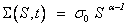 ,
 .
This process was discussed by Cox and Ross [5] as an alternative to the Black-Scholes model. The constant should now have units
of  per
√(annum) so, for example, one could multiply a Black-Scholes volatility
by the relevant power of today’s underlying price to get a sensible number: if
 , and if the Black-Scholes volatility is 20% (per
√(annum)) and the current price of the underlying is $100, then would be of the order
of 4√(dollars) (per √(annum)).
Shifted lognormal
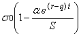 ,
 .
This is a “shifted” version of the lognormal process
and has been discussed in, e.g., [4] (a displaced diffusion model was first discussed by
Rubinstein [15]). As for that
case, the constant  is a percentage
per √(annum), and
 should have
units of . To avoid
negative values of , we further demand that
 in this process.
For these functions, the user need only enter the relevant
parameters to define the local volatility ( for the lognormal and normal processes; and for the CEV and
shifted lognormal processes).
On the other hand, the FINCAD functions aaOption_LVtbl_p,
aaOption_LVtbl_payoff_p,
and aaOption_LVtbl_iv
allow the user to specify an arbitrary local volatility function. This is done by giving a table of the form:
vol_tbl
|
time t |
underlying S |
local volatility
Σ(S,t) |
|
|
|
|
|
… |
… |
… |
|
|
|
|
|
|
|
|
|
… |
… |
… |
|
|
|
|
|
… |
… |
… |
|
|
|
|
|
… |
… |
… |
|
|
|
|


where, in each row, the local volatility function is
given for that particular value of time and underlying asset price. The numerical techniques used to value
options within such a user-defined process are described below. It is important to realize that these
techniques involve an interpolation, and possibly an extend on the values given
in the vol_tbl.
There are three distinct interpolation methods available
through the interp_vol switch: bi-linear, bi-cubic and thin plate. The bi-linear and bi-cubic methods involve
two one-dimensional interpolations, first interpolating in the direction, and
then in the direction. On the other hand, the thin plate method involves
constructing directly a two-dimensional surface through all the given data
points[4]. Either way, the more distinct points given in
the vol_tbl, the better will be the accuracy of the interpolation method.
If values of the local volatility are needed that lie
outside of the given ranges of and in the vol_tbl,
then an extrapolation will also be performed.
The bi-linear and bi-cubic methods will extend to constant values of the
local volatility, whereas the thin plate method will extrapolate to values of
the local volatility that are linear in and/or .
Pricing Methodology
The suite of functions described in this document allow
the user to compute the price and risk statistics for plain vanilla options,
binary options (digital all-or-nothing calls or puts), a portfolio of plain
vanillas, a host of trading strategies (listed in the Appendix) and options
with arbitrary piecewise linear payoff functions.
The functions which deal solely with European options and
the pre-defined local volatility functions (aaOption_LV_eu_p, aaOption_LV_payoff_eu_p
and aaOption_LV_iv),
use only closed form solutions. All
other functions use numerical finite-difference methods on the no-arbitrage PDE
(Equation
1) to compute the price and risk statistics of the
options, portfolios or strategies.
Closed-Form Solutions
For European plain vanilla options within the pre-defined
processes discussed above, closed-form solutions of Equation 1 exist[5]
and are implemented by the FINCAD functions aaOption_LV_eu_p, aaOption_LV_payoff_eu_p
and aaOption_LV_iv. For a portfolio or trading strategy built up
from such plain vanillas, these formulae are simply applied to the individual
components of the portfolio or strategy in the appropriate manner. For the function aaOption_LV_payoff_eu_p,
the (piecewise linear) user-defined payoff is first decomposed into its
constituent European plain vanilla calls and puts, then each are priced
individually. Defining and  as the
valuation and maturity dates respectively, and
 as the underlying
price on the valuation date, the relevant solutions are:
Lognormal
In this case the function aaOption_LV_eu_p
simply uses the Black-Scholes formulae by internally calling aaBSG
or – in the case of a binary option – aaDigital_AON. The prices of a call () and put ( ) option are:
 ,
 ,
and those of a Binary call ( ) and Binary put (
 ) option are:
 ,
 ,
where:
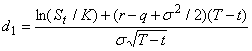 ,
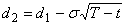 , and
 is the cumulative
normal distribution.
See the Black-Scholes Generalized and the Binary Options FINCAD Math
Reference documents for further details of these functions.
Normal
The prices of a call () and put () option in this case are:
 ,
 .
where
 is the standard normal
probability density function, and
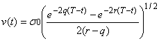 ,
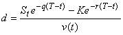 .
CEV
The solutions in this case (see, e.g., [10]) depend on the parameter . For  , the prices of a call () and a put () option are:
 ,
 .
For  we instead have:
 ,
 ,
where  denotes the cumulative
non-central chi-squared distribution, with
 degrees of
freedom and non-centrality parameter
 ,
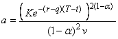 ,
 ,
 ,
and
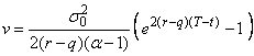 .
The non-central chi-squared function can be computed
numerically using a well-known algorithm [7]. This formally
involves an infinite sum of terms which, in practice, is terminated upon
reaching a required level of accuracy within some maximum number of
iterations. Of course, the procedure
could fail if the level of accuracy is not reached within this maximum number.
Shifted lognormal
The solutions within this process (see, e.g., [4]) can be had from the standard Black-Scholes formulae
above, with  replaced by
 and with
 replaced by
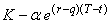 , so again the function aaOption_LV_eu_p
simply internally calls aaBSG (for plain vanilla options) or aaDigital_AON
(for binary options). Note that these
solutions hold only under the assumptions that
 and
 , so we demand that the inputs satisfy these conditions.
In each of these processes, the Greeks are also given by
closed-form expressions, the derivatives of the option price with respect to
the relevant quantity. The sensitivities
to changes in the rates are taken in one of two ways: if the user enters a
single rate with a specific compounding and/or accrual method, then the
sensitivity is with respect to the given type of rate and accrual method. If, on the other hand, the user enters a
discount factor curve, then the sensitivity is with respect to the annually
compounded rate with an actual/365 (fixed) accrual factor. The only remaining subtlety is that – for the
normal and CEV processes – we take vega to be the sensitivity with respect to
the local volatility:

 ,
so that the functions return

 ,

 ,
in these cases.
Finite-Difference Methods
The FINCAD functions aaOption_LV_p, aaOption_LVtbl_p,
aaOption_LV_payoff_p,
aaOption_LVtbl_payoff_p
and aaOption_LVtbl_iv
all use finite difference methods on the no-arbitrage PDE (Equation 1). More
specifically, they use the Crank-Nicolson scheme which is unconditionally
stable (the von Neumann stability criterion is discussed in [1]) and has the best convergence properties as compared
to the fully implicit or fully explicit schemes. For a discussion of the general procedure
see, e.g., [16] and for an application to local volatility models,
see [1].
All finite-difference methods involve discretizing the
time and underlying directions in the no-arbitrage PDE Equation 1,
and approximating the derivative terms in various ways. Since the equation is a (backward) parabolic
PDE, it has a unique solution given an initial condition (really a final
condition since time runs backwards) and some boundary conditions. In the case at hand, the initial condition is
just the final payoff of the option, and various sensible boundary conditions
can be used (see, e.g., [16] for a discussion of possible boundary conditions).
The first step is to set up a grid in which time runs from
the valuation date to the maturity date of the option, and we set the minimum
and maximum values of the underlying asset in such a way as to capture most of
the possible movements in the asset price.
As discussed in [1], it is possible to set the grid size such that the
(risk-neutral) probability of the underlying price at maturity falling outside
the grid is roughly 0.01%. To ensure
this for the lognormal process, we take:
 ,
 .
For the shifted lognormal process, we use the
same expressions but with replaced by and for the CEV
process we take to be an at-the-money
“effective lognormal volatility”. For
the user-defined process, we instead take  and
 to be the above
expressions, but with given the average
value of the volatility entered by the user in the vol_tbl input. In all these cases except the shifted
lognormal process with negative , the underlying price will be strictly positive[6]. Finally, for the normal process we take:
 ,
 ,
which does allow for negative values of the underlying
price, if the volatility is sufficiently large with respect to . Whilst not
appropriate for equity derivatives, the normal process does allow for negative
values of the underlying, and to match with the closed form solutions for the
European call and put option, the numerical procedure should likewise allow for
negative values. In all cases, we
further arrange the grid such that the present price of the underlying asset
lies exactly on a row of grid points.
Let us assume that our grid has  equally spaced
steps in the underlying direction, labeled by
 and
 equally spaced
steps in the time direction, labeled by
 . The (discrete)
values of time and underlying price are thus given by:
 ,
 ,
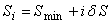 ,
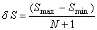 .
The Crank-Nicolson scheme uses the following
approximations for the derivatives in Equation
1:
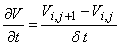 ,
 ,
 .
It can be shown that the error in these
expressions is  , which is better than either the fully implicit or
fully explicit schemes.
We proceed by substituting these approximations
into Equation
1 and re-arranging to give the matrix equation:
 ,
where
 denotes the vector of
option prices at time step
 as a function
of the underlying price,
 is a known matrix (at
that time step) and
 is a vector which
contains the boundary conditions at the edges of the lattice.
Given that we know the payoff function, we can step
backwards in time from the maturity to the valuation date, solving this matrix
equation at each time step. Since the
matrix on the left hand side of the equation turns out to be tridiagonal, there
are very efficient ways to do this [13]. In the
European case, we solve the equation using the method of LU decomposition,
although for American options we have to solve the equation iteratively, at
each grid point assessing whether or not exercise of the option is optimal; we
use the method of successive over-relaxation (SOR) to do this[7].
If the present value of the underlying is equal to  then the fair
value of the option is just
 , the
 element of
 . With the above
approximations for the derivatives, the Greeks
 ,
 and
 are given by the
expressions:
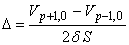 ,
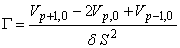 ,
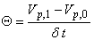 .
The remaining Greeks  (with respect
to both the risk-free rate and the dividend yield) and vega, are calculated by
bumping the relevant quantities and re-valuing the option. For both the risk-free rate and the dividend
yield, is taken to be
the sensitivity with respect to a 1% change in the type of rate and/or accrual
method that the user supplies (if a single rate is given), or to a 1% change in
the annually compounded rate with accrual factor actual/365 (fixed) if the user
supplies a discount factor curve.
Finally, it should be noted that we take vega to be the sensitivity with
respect to a 1% change in the local volatility.
In the user-defined case, we thus bump each point in the vol_tbl by
1%. For both the lognormal and shifted
lognormal processes, we bump the parameter by 1%; for the
normal process we instead bump the parameter by
 ; and for the CEV process we bump the parameter by
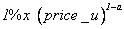 . For more details
about the calculation of Greeks, see the Greeks of Options on Non-Interest Rate Instruments
FINCAD Math Reference document.
In the European case, we can value a portfolio of options,
a trading strategy, or an option with an arbitrary payoff function all in one
go, since option exercise is only possible on the maturity date. We first construct a (piecewise linear)
payoff function for the various strategies, the user-defined portfolio or the
user-defined payoff, and then solve Equation
1 using this payoff function as the “initial”
condition. In the American case,
however, we have to value the options individually, since they can be exercised
independently of each other[8].
There is a well-known stability criterion for the
Crank-Nicolson method which is important to consider when the volatilities are
small and/or the rates are large [8]. To avoid
spurious numerical results, the step size in the underlying direction should be
such that:
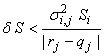 ,
which should hold at every time step. This condition gives rise to a minimum number
of S_steps if such problems[9]
are to be avoided – the “minimum S_steps” statistics in the Description of Outputs section. Unless the volatility is very small and/or
the rates are very large, the minimum number of S_steps is of order 1 to 10, so
this issue will not be a problem. We
still recommend that a relatively large number of steps is used so the “minimum
S_steps” output is at least 200 S_steps (the minimum S_steps statistic will
thus only give the true minimum number if it is greater than 200). Note also that the function aaOption_LVtbl_iv
does not output this number.
FINCAD Functions
aaOption_LV_p
(price_u, payoff_type, strike_tbl, option_style, d_exp, d_v, process,
param_tbl, df_crv_std, df_crv_hld, intrp, S_steps, t_steps, numerical method,
stat)
Calculates the price and risk statistics of a standard
option, a standard option strategy, or an option portfolio, for a parameterized
local volatility function such as those which define the lognormal, normal, CEV
and shifted lognormal stochastic processes.
The function uses finite difference methods on the underlying
no-arbitrage PDE, and handles European and American exercise features.
aaOption_LVtbl_p
(price_u, payoff_type, strike_tbl, option_style, d_exp, d_v, vol_tbl,
interp_vol, df_crv_std, df_crv_hld, intrp, S_steps, t_steps, numerical method,
stat)
Calculates the price and risk statistics of a standard
option, a standard option strategy, or an option portfolio, given a
user-defined local volatility function.
The function uses finite difference methods on the underlying
no-arbitrage PDE, and handles European and American exercise features.
aaOption_LV_payoff_p
(price_u, payoff_tbl, option_style, d_exp, d_v, process, param_tbl, df_crv_std,
df_crv_hld, intrp, S_steps, t_steps, numerical method, stat)
Calculates the price and risk statistics of an option with
a freestyle payoff, for a parameterized local volatility function such as those
which define the lognormal, normal, CEV and shifted lognormal stochastic processes. The function uses finite difference methods
on the underlying no-arbitrage PDE, and handles European and American exercise
features.
aaOption_LVtbl_payoff_p
(price_u, payoff_tbl, option_style, d_exp, d_v, vol_tbl, interp_vol,
df_crv_std, df_crv_hld, intrp, S_steps, t_steps, numerical method, stat)
Calculates the price and risk statistics of an option with
a freestyle payoff, given a user-defined local volatility function. The function uses finite difference methods
on the underlying no-arbitrage PDE, and handles European and American exercise
features.
aaOption_LV_eu_p
(price_u, payoff_type, strike_tbl, d_exp, d_v, process, param_tbl, df_crv_std,
df_crv_hld, intrp, stat)
Calculates the price and risk statistics of a European
plain vanilla call or put option, a standard European option strategy, or a
user-defined portfolio of European plain vanilla options, for a parameterized
local volatility function such as those which define the lognormal, normal, CEV
and shifted lognormal stochastic processes.
The function uses closed-form solutions for standard processes.
aaOption_LV_payoff_eu_p
(price_u, payoff_tbl, d_exp, d_v, process, param_tbl, df_crv_std, df_crv_hld,
intrp, stat)
Calculates the price and risk statistics of an option with
a freestyle payoff, for a parameterized local volatility function such as those
which define the lognormal, normal, CEV and shifted lognormal stochastic
processes. The function uses closed-form
solutions for standard processes.
aaOption_LV_iv
(price_u, TK_tbl, d_v, process, param_tbl, df_crv_std, df_crv_hld, intrp)
Plots the implied volatility smile, for a parameterized
local volatility function such as those which define the lognormal, normal, CEV
and shifted lognormal stochastic processes.
The function uses closed-form solutions for standard processes.
aaOption_LVtbl_iv
(price_u, TK_tbl, d_v, vol_tbl, interp_vol, df_crv_std, df_crv_hld, intrp,
S_steps, t_steps, numerical method)
Plots the implied volatility smile, given a user-defined local
volatility function. The function uses
finite difference methods on the underlying no-arbitrage PDE.
Description of Inputs
aaOption_LV_p
|
Input Argument |
Type |
Description |
|
price_u |
number |
current value of the underlying stock |
|
payoff_type |
number |
switch to select the payoff of the option/strategy 1. portfolio
(user-defined), 2. vanilla
call, 3. vanilla
put, 4. binary
call, 5. binary
put, 6. call
(bull) spread, 7. put
(bear) spread, 8. risk
reversal (collar), 9. seagull,
10. straddle,
11. strangle,
12. guts,
13. butterfly,
14. condor,
15. iron
butterfly, 16. iron
condor, 17. box,
18. ratio
call spread, 19. ratio
put spread, 20. synthetic
forward, 21. participating
forward (put), 22. participating
forward (call), 23. call
ladder, 24. put
ladder, 25. call
spread vs. put, 26. put
spread vs. call, 27. straddle
vs. call, 28. straddle
vs. put. The choice will affect the form of the
strike_tbl input. |
|
strike_tbl |
table or number |
table of (possibly time-varying) strikes to define the
option, portfolio or strategy; see below for details |
|
option_style |
number |
switch to select the option style (European,
American). If option_style = American
then all the options in the portfolio or strategy can be exercised
independently. |
|
d_exp |
date |
maturity date of the option |
|
d_v |
date |
valuation date |
|
process |
number |
switch to select the local volatility function (lognormal,
normal, CEV, shifted lognormal). The
choice will affect the form of the param_tbl input. |
|
param_tbl |
table or number |
table of parameters to define the local volatility
function; see below for details |
|
df_crv_std |
table or rate |
risk-free discount factor curve. The discount factor curve may be input as an
N×2 table (column 1 = date, column 2 = discount factor), or as a single cell
containing a rate. If input as a single rate, there are three format choices:
1.
a rate (1×1 table); or 2. a
rate and a rate quotation basis as per Switch 43 (1×2 table); or 3. a
rate, a rate quotation basis, and an accrual method as per Switch 331 (1×3
table). If the basis or accrual method are not
provided, they are assumed to be annual, actual/365. An N×2 flat-rate discount factor curve is
constructed internally between the value date and the expiry date, using the
rate, basis and accrual method. |
|
df_crv_hld |
table or rate |
dividend discount factor curve. The discount factor curve may be input as an
N×2 table (column 1 = date, column 2 = discount factor), or as a single cell
containing a rate. If input as a single rate, there are three format choices:
1.
a rate (1×1 table); or 2. a
rate and a rate quotation basis as per Switch 43 (1×2 table); or 3. a
rate, a rate quotation basis, and an accrual method as per Switch 331 (1×3
table). If the basis or accrual method are not
provided, they are assumed to be annual, actual/365. An N×2 flat-rate discount factor curve is
constructed internally between the value date and the expiry date, using the
rate, basis and accrual method. |
|
intrp |
number |
switch to select which interpolation method to use on the
discount factor curves (linear, cubic spline, exponential, linear spot rates) |
|
S_steps |
number |
number of steps to use in the underlying (S) direction |
|
t_steps |
number |
number steps to use in the time (t) direction |
|
numerical method |
table or number |
switch to select which numerical method to use to solve
the PDE (currently only Crank-Nicolson is implemented) |
|
stat |
table or number |
switch to select which output the user wants; see Description of Outputs section |
aaOption_LVtbl_p
|
Input Argument |
Type |
Description |
|
price_u |
number |
current value of the underlying stock |
|
payoff_type |
number |
switch to select the payoff of the option/strategy 1.
portfolio (user-defined), 2. vanilla
call, 3. vanilla
put, 4. binary
call, 5. binary
put, 6. call
(bull) spread, 7. put
(bear) spread, 8. risk
reversal (collar), 9. seagull,
10. straddle,
11. strangle,
12. guts,
13. butterfly,
14. condor,
15. iron
butterfly, 16. iron
condor, 17. box,
18. ratio
call spread, 19. ratio
put spread, 20. synthetic
forward, 21. participating
forward (put), 22. participating
forward (call), 23. call
ladder, 24. put
ladder, 25. call
spread vs. put, 26. put
spread vs. call, 27. straddle
vs. call, 28. straddle
vs. put. The choice will affect the form of the
strike_tbl input. |
|
strike_tbl |
table or number |
table of (possibly time-varying) strikes to define the
option, portfolio or strategy; see below for details |
|
option_style |
number |
as above |
|
d_exp |
date |
maturity date of the option |
|
d_v |
date |
valuation date |
|
vol_tbl |
table |
table to define the local volatility function. This is an N×3 table (column 1 = time,
column 2 = underlying, column 3 = local volatility for that value of time and
underlying). The time values can be
entered as dates or as time in years since d_v. The more values entered the better, since
an interpolation on the table must be performed to generate the local
volatility on each node of the grid.
|
|
interp_vol |
number |
switch to select which interpolation method to use on
vol_tbl (bi-linear, bi-cubic, thin plate) |
|
df_crv_std |
table or rate |
as above |
|
df_crv_hld |
table or rate |
as above |
|
intrp |
number |
as above |
|
S_steps |
number |
number of steps to use in the underlying (S) direction |
|
t_steps |
number |
number steps to use in the time (t) direction |
|
numerical method |
table or number |
switch to select which numerical method to use to solve
the PDE (currently only Crank-Nicolson is implemented) |
|
stat |
table or number |
switch to select which output the user wants; see Description of Outputs section |
aaOption_LV_payoff_p
|
Input Argument |
Type |
Description |
|
price_u |
number |
current value of the underlying stock |
|
payoff_tbl |
table |
table defining the payoff profile. This is an N×2 table (column 1 =
underlying, column 2 = payoff) specifying the payoff at various values of the
underlying. A piecewise linear payoff
function is constructed internally from this data, so it is important to
enter all the points necessary to construct the correct (piecewise linear)
payoff. |
|
option_style |
number |
as above |
|
d_exp |
date |
maturity date of the option |
|
d_v |
date |
valuation date |
|
process |
number |
switch to select the local volatility function (lognormal,
normal, CEV, shifted lognormal). The
choice will affect the form of the param_tbl input. |
|
param_tbl |
table or number |
table of parameters to define the local volatility
function; see below for details |
|
df_crv_std |
table or rate |
as above |
|
df_crv_hld |
table or rate |
as above |
|
intrp |
number |
as above |
|
S_steps |
number |
number of steps to use in the underlying (S) direction |
|
t_steps |
number |
number steps to use in the time (t) direction |
|
numerical method |
table or number |
switch to select which numerical method to use to solve
the PDE (currently only Crank-Nicolson is implemented) |
|
stat |
table or number |
switch to select which output the user wants; see Description of Outputs section |
aaOption_LVtbl_payoff_p
|
Input Argument |
Type |
Description |
|
price_u |
number |
current value of the underlying stock |
|
payoff_tbl |
table |
table defining the payoff profile. This is an N×2 table (column 1 =
underlying, column 2 = payoff) specifying the payoff at various values of the
underlying. A piecewise linear payoff
function is constructed internally from this data, so it is important to
enter all the points necessary to construct the correct (piecewise linear)
payoff. |
|
option_style |
number |
as above |
|
d_exp |
date |
maturity date of the option |
|
d_v |
date |
valuation date |
|
vol_tbl |
table |
table to define the local volatility function. This is an N×3 table (column 1 = time,
column 2 = underlying, column 3 = local volatility for that value of time and
underlying). The time values can be
entered as dates or as time in years since d_v. The more values entered the better, since
an interpolation on the table must be performed to generate the local
volatility on each node of the grid.
|
|
interp_vol |
number |
switch to select which interpolation method to use on
vol_tbl (bi-linear, bi-cubic, thin plate) |
|
df_crv_std |
table or rate |
as above |
|
df_crv_hld |
table or rate |
as above |
|
intrp |
number |
as above |
|
S_steps |
number |
number of steps to use in the underlying (S) direction |
|
t_steps |
number |
number steps to use in the time (t) direction |
|
numerical method |
table or number |
switch to select which numerical method to use to solve
the PDE (currently only Crank-Nicolson is implemented) |
|
stat |
table or number |
switch to select which output the user wants; see Description of Outputs section |
aaOption_LV_eu_p
|
Input Argument |
Type |
Description |
|
price_u |
number |
current value of the underlying stock |
|
payoff_type |
number |
switch to select the payoff of the option/strategy 1.
portfolio (user-defined), 2. vanilla
call, 3. vanilla
put, 4. binary
call, 5. binary
put, 6. call
(bull) spread, 7. put
(bear) spread, 8. risk
reversal (collar), 9. seagull,
10. straddle,
11. strangle,
12. guts,
13. butterfly,
14. condor,
15. iron
butterfly, 16. iron
condor, 17. box,
18. ratio
call spread, 19. ratio
put spread, 20. synthetic
forward, 21. participating
forward (put), 22. participating
forward (call), 23. call
ladder, 24. put
ladder, 25. call
spread vs. put, 26. put
spread vs. call, 27. straddle
vs. call, 28. straddle
vs. put. The choice will affect the form of the
strike_tbl input. |
|
strike_tbl |
table or number |
table of (possibly time-varying) strikes to define the
option, portfolio or strategy; see below for details |
|
d_exp |
date |
maturity date of the option |
|
d_v |
date |
valuation date |
|
process |
number |
switch to select the local volatility function (lognormal,
normal, CEV, shifted lognormal). The
choice will affect the form of the param_tbl input. |
|
param_tbl |
table or number |
table of parameters to define the local volatility
function; see below for details |
|
df_crv_std |
table or rate |
as above |
|
df_crv_hld |
table or rate |
as above |
|
intrp |
number |
as above |
|
stat |
table or number |
switch to select which output the user wants; see Description of Outputs section |
aaOption_LV_payoff_eu_p
|
Input Argument |
Type |
Description |
|
price_u |
number |
current value of the underlying stock |
|
payoff_tbl |
table |
table defining the payoff profile. This is an N×2 table (column 1 =
underlying, column 2 = payoff) specifying the payoff at various values of the
underlying. A piecewise linear payoff
function is constructed internally from this data, so it is important to
enter all the points necessary to construct the correct (piecewise linear)
payoff. |
|
d_exp |
date |
maturity date of the option |
|
d_v |
date |
valuation date |
|
process |
number |
switch to select the local volatility function (lognormal,
normal, CEV, shifted lognormal). The
choice will affect the form of the param_tbl input. |
|
param_tbl |
table or number |
table of parameters to define the local volatility
function; see below for details |
|
df_crv_std |
table or rate |
as above |
|
df_crv_hld |
table or rate |
as above |
|
intrp |
number |
as above |
|
stat |
table or number |
switch to select which output the user wants; see Description of Outputs section |
aaOption_LV_iv
|
Input Argument |
Type |
Description |
|
price_u |
number |
current value of the underlying stock |
|
TK_tbl |
table |
table of option maturity dates and exercise prices for
which to return the implied volatility |
|
d_v |
date |
valuation date |
|
process |
number |
switch to select the local volatility function (lognormal,
normal, CEV, shifted lognormal). The
choice will affect the form of the param_tbl input. |
|
param_tbl |
table or number |
table of parameters to define the local volatility
function; see below for details |
|
df_crv_std |
table or rate |
as above |
|
df_crv_hld |
table or rate |
as above |
|
intrp |
number |
as above |
aaOption_LVtbl_iv
|
Input Argument |
Type |
Description |
|
price_u |
number |
current value of the underlying stock |
|
TK_tbl |
table |
table of option maturity dates and exercise prices for
which to return the implied volatility |
|
d_v |
date |
valuation date |
|
vol_tbl |
table |
table to define the local volatility function. This is an N×3 table (column 1 = time,
column 2 = underlying, column 3 = local volatility for that value of time and
underlying). The time values can be
entered as dates or as time in years since d_v. The more values entered the better, since
an interpolation on the table must be performed to generate the local
volatility on each node of the grid.
|
|
interp_vol |
number |
switch to select which interpolation method to use on
vol_tbl (bi-linear, bi-cubic, thin plate) |
|
df_crv_std |
table or rate |
as above |
|
df_crv_hld |
table or rate |
as above |
|
intrp |
number |
as above |
|
S_steps |
number |
number of steps to use in the underlying (S) direction |
|
t_steps |
number |
number steps to use in the time (t) direction |
|
numerical method |
table or number |
switch to select which numerical method to use to solve the
PDE (currently only Crank-Nicolson is implemented) |
|
stat |
table or number |
switch to select which output the user wants; see Description of Outputs section |
param_tbl
In more detail, the local volatility function in aaOption_LV_p,
aaOption_LV_payoff_p,
aaOption_LV_eu_p
and aaOption_LV_iv
is specified through the process and param_tbl inputs. They must take one of the following forms:
·
if process = lognormal
or normal, only one parameter must be specified
param_tbl
|
volatility |
|
|
·
if process = CEV or
shifted lognormal, two parameters must be specified
param_tbl
|
vlt |
parameter |
|
|
|
strike_tbl
The various options/portfolios/strategies in the functions
aaOption_LV_p,
aaOption_LVtbl_p
and aaOption_LV_eu_p
are specified through the payoff_type and strike_tbl inputs. The various strategies FINCAD supports are
all described in [11], where P&L diagrams can also be found; see the
Appendix for a breakdown into their constituent plain vanillas. The strike_tbl should specify the relevant
exercise prices, and must take one of the following forms.
·
if payoff_type = portfolio
(user-defined), the details of
the options in the portfolio must be specified.
strike_tbl
|
long/short |
call/put |
strike |
|
|
1/2 |
|
|
|
1/2 |
|
|
… |
… |
… |
|
|
1/2 |
|


Here,  denotes respectively a
long/short position in
 options, which are
either calls (1) or puts (2), with the given strikes. The individual options must be either all
European or all American.
·
if payoff_type = vanilla
call, vanilla put, straddle or synthetic forward, only a single exercise
price must be entered.
strike_tbl
|
exercise price |
|
|
·
if payoff_type = vanilla
call or vanilla put (and if option_style = American), a time-varying
exercise price can also be specified.
strike_tbl
|
effective date |
terminating date |
exercise price |
|
|
|
|
|
|
|
|
|
… |
… |
… |
|
|
|
|


where
each terminating date must be greater than the
corresponding effective date  and
each effective date must be greater than or equal to
the previous terminating date 
By allowing for gaps in this table, blackout periods
are thus allowed (alternatively, a blackout period can be specified by setting  ).
·
if payoff_type = binary
call or binary put, a single
exercise price and a cash payout must be specified.
strike_tbl
|
exercise price |
cash payout |
|
|
|
The binaries are digital all-or-nothing options,
which pay a fixed amount of cash (and can be European or American).
·
if payoff_type = participating
forward (put) or participating forward (call), a single exercise price and a percentage (the degree of
participation) must be specified.
strike_tbl
|
exercise price |
percentage |
|
|
|

·
if payoff_type = straddle
vs. call or straddle vs. put, then
two distinct exercise prices must be specified
strike_tbl
|
exercise price 1 |
exercise price 2 |
|
|
|

·
if payoff_type = call (bull) spread, put (bear)
spread, risk reversal (collar), strangle, guts, butterfly, condor, box, then two
distinct exercise prices must be specified.
strike_tbl
|
exercise price 1 |
exercise price 2 |
|
|
|
where the restriction  applies.
·
if payoff_type = call
spread vs. put or put spread vs. call,
then three distinct exercise prices must be specified.
strike_tbl
|
exercise price 1 |
exercise price 2 |
exercise price 3 |
|
|
|
|
where the restriction applies.
·
if payoff_type = seagull,
iron butterfly, call ladder, put ladder, then three distinct exercise prices must be specified.
strike_tbl
|
exercise price 1 |
exercise price 2 |
exercise price 3 |
|
|
|
|
where the restriction  applies.
·
if payoff_type = ratio
call spread or ratio put spread,
then two exercise prices and two integers must be specified (the integers give
the ratio of the spread).
strike_tbl
|
exercise price 1 |
exercise price 2 |
number 1 |
number 2 |
|
|
|
|
|


where the restrictions  and
 apply.
·
if payoff_type = iron
condor then four distinct exercise prices must be specified.
strike_tbl
|
strike 1 |
strike 2 |
strike 3 |
strike 4 |
|
|
|
|
|

where the restriction  applies.
payoff_tbl
The functions aaOption_LV_payoff_p,
aaOption_LV_payoff_eu_p
and aaOption_LVtbl_payoff_p
allow the user to specify an arbitrary (piecewise linear) payoff function. This is done through the payoff_tbl input
which must take the following form:
payoff_tbl
|
underlying |
payoff |
|
|
|
|
|
|
|
… |
… |
|
|
|


where the payoff  is given for a set of
underlying values
 . A piecewise linear
payoff function is constructed from this data internally, so it is important
that the user enter enough points to construct the payoff of interest. Outside of the range of given underlying
values, the payoff is constructed by linear extrapolation from the last two (or
first two) points in the payoff_tbl.
Description of Outputs
aaOption_LV_p, aaOption_LVtbl_p , aaOption_LV_payoff_p,
aaOption_LVtbl_payoff_p, aaOption_LV_smile_p, aaOption_LV_smile_payoff_p
These functions output the price and risk statistics of
the relevant option, strategy or portfolio.
There is one additional output, which is the minimum suggested number of
steps in the underlying direction; this is discussed in the Finite Difference section above.
|
Output Statistics |
Type |
Description |
|
fair value |
number |
fair value of the option. |
|
delta |
number |
rate of change in the fair value of the option per change
in the current value of the underlying stock.
This is the derivative of the option price with respect to the current
value of the underlying. |
|
gamma |
number |
rate of change in the value of delta per change in the
current value of the underlying stock.
This is the second derivative of the option price with respect to the
current value of the underlying. |
|
theta |
number |
rate of change in the fair value of the option per one day
decrease in the option time. This is
the negative of the derivative of the option price with respect to the option
time (in years), divided by 365. |
|
vega |
number |
rate of change in the fair value of the option per 1%
change in annual volatility. This is
the derivative of the option price with respect to the annual volatility,
divided by 100. |
|
rho of rate |
number |
rate of change in the fair value of the option per 1%
change in the risk-free rate. This is
the derivative of the option price with respect to the risk-free rate,
divided by 100. |
|
rho of holding cost |
number |
rate of change in the fair value of the option per 1%
change in the dividend rate. This is
the derivative of the option price with respect to the dividend rate, divided
by 100. |
|
minimum S_steps |
number |
the minimum suggested number of S_steps |
aaOption_LV_eu_p, aaOption_LV_payoff_eu_p
These functions output the price and risk statistics of
the relevant option, strategy or portfolio.
|
Output Statistics |
Type |
Description |
|
fair value |
number |
fair value of the option. |
|
delta |
number |
rate of change in the fair value of the option per change
in the current value of the underlying stock.
This is the derivative of the option price with respect to the current
value of the underlying. |
|
gamma |
number |
rate of change in the value of delta per change in the
current value of the underlying stock.
This is the second derivative of the option price with respect to the
current value of the underlying. |
|
theta |
number |
rate of change in the fair value of the option per one day
decrease in the option time. This is
the negative of the derivative of the option price with respect to the option
time (in years), divided by 365. |
|
vega |
number |
rate of change in the fair value of the option per 1%
change in annual volatility. This is
the derivative of the option price with respect to the annual volatility,
divided by 100. |
|
rho of rate |
number |
rate of change in the fair value of the option per 1%
change in the risk-free rate. This is
the derivative of the option price with respect to the risk-free rate,
divided by 100. |
|
rho of holding cost |
number |
rate of change in the fair value of the option per 1%
change in the dividend rate. This is
the derivative of the option price with respect to the dividend rate, divided
by 100. |
aaOption_LV_iv, aaOption_LVtbl_iv
These functions will output a table of implied
volatilities for the strikes and maturities given in the TK_tbl input. The results can be plotted to give an implied
volatility surface. The output table
will be of the following form (the first two columns are just the TK_tbl
input):
output_smile_tbl
|
maturity |
exercise price |
implied volatility |
|
|
|
|
|
… |
… |
… |
|
|
|
|
|
|
|
|
|
… |
… |
… |
|
|
|
|
|
… |
… |
… |
|
|
|
|
|
… |
… |
… |
|
|
|
|


where the  are implied volatilities for maturity
 and exercise
price
 .
Examples
Example 1: American Call within the
Lognormal model
Today is January 1, 2007.
Consider an at-the-money American call option that matures 6 months from
today. It has an exercise price of $50
for the life of the option. The current
underlying price is $50, the estimated annual volatility of the underlying is
20%, the risk-free rate is 7.5% (annual compounding, actual/365 accrual), and
the dividend rate is 2.5% (annual compounding, actual/365 accrual).
Suppose we want to value the option with the assumption
that the underlying asset undergoes a lognormal evolution (i.e., within the
standard Black-Scholes model). There are
various ways to do this with the FINCAD functions described above.
The most direct valuation is to call aaOption_LV_p
with the following inputs:
aaOption_LV_p
|
Argument |
Description |
Example Data |
Switch |
Comments |
|
price_u |
underlying price |
50 |
|
|
|
payoff_type |
payoff type |
2 |
vanilla call |
|
|
strike_tbl |
strike table |
50 |
|
a single strike to define the call |
|
option_style |
option style |
2 |
American |
|
|
d_exp |
expiry date |
1-Jul-2007 |
|
6 months from today |
|
d_v |
value date |
1-Jan-2007 |
|
|
|
process |
local volatility function |
1 |
lognormal |
|
|
param_tbl |
parameters for the local volatility function |
20% |
|
|
|
df_crv_std |
discount factor curve – risk free |
7.5% |
|
annual compounding and actual/365 accrual is assumed |
|
df_crv_hld |
discount factor curve – holding cost |
2.5% |
|
annual compounding and actual/365 accrual is assumed |
|
intrp |
interpolation method |
3 |
exponential |
not used for constant rates |
|
S_steps |
number of underlying steps |
200 |
|
|
|
t_steps |
number of time steps |
200 |
|
|
|
scheme |
numerical method |
1 |
Crank-Nicolson |
|
|
stat |
list of statistics |
1…8 |
|
|
With these inputs, the results are:
Results
|
Output Statistics |
Description |
Value |
|
1 |
fair value |
3.346566596 |
|
2 |
delta |
0.586012281 |
|
3 |
gamma |
0.054418608 |
|
4 |
theta |
-0.010589312 |
|
5 |
vega |
0.1348654 |
|
6 |
rho of rate |
0.11962665 |
|
7 |
rho of holding cost |
-0.142776752 |
|
8 |
minimum S_steps |
200 |
Since the minimum suggested number of S_steps is
200, we know that the inputs are such that we need less than 200 S_steps to
avoid any unstable numerical results; however, a minimum of 200 steps is always
recommended.
To understand some of the features of the other
FINCAD functions described here we can, for example, check the above results
with a user-defined local volatility function (that is equal to a constant of
20%). To do this, call aaOption_LVtbl_p
with the following inputs:
aaOption_LVtbl_p
|
Argument |
Description |
Example Data |
Switch |
Comments |
|
price_u |
underlying price |
50 |
|
|
|
payoff_type |
payoff type |
2 |
vanilla call |
|
|
strike_tbl |
strike table |
50 |
|
a single strike to define the call |
|
option_style |
option style |
2 |
American |
|
|
d_exp |
expiry date |
1-Jul-2007 |
|
6 months from today |
|
d_v |
value date |
1-Jan-2007 |
|
|
|
vol_tbl |
volatility table |
see below |
|
a user-defined lognormal process |
|
interp_vol |
interpolation method for vol_tbl |
1 |
bi-linear |
since the local volatility is constant, the choice will
not affect the results |
|
df_crv_std |
discount factor curve – risk free |
7.5% |
|
annual compounding and actual/365 accrual is assumed |
|
df_crv_hld |
discount factor curve – holding cost |
2.5% |
|
annual compounding and actual/365 accrual is assumed |
|
intrp |
interpolation method |
3 |
exponential |
not used for constant rates |
|
S_steps |
number of underlying steps |
200 |
|
|
|
t_steps |
number of time steps |
200 |
|
|
|
scheme |
numerical method |
1 |
Crank-Nicolson |
|
|
stat |
list of statistics |
1…8 |
|
|
Since the local volatility we want to define is a
constant, there is no need to specify too many distinct points in the vol_tbl:
vol_tbl
|
time |
underlying |
local volatility |
|
1-Jan-2006 |
20 |
20% |
|
1-Jan-2006 |
50 |
20% |
|
1-Jan-2006 |
80 |
20% |
|
1-Apr-2006 |
20 |
20% |
|
1-Apr-2006 |
50 |
20% |
|
1-Apr-2006 |
80 |
20% |
|
1-Jul-2006 |
20 |
20% |
|
1-Jul-2006 |
50 |
20% |
|
1-Jul-2006 |
80 |
20% |
With these inputs, the results are as for aaOption_LV_p
above.
Since the call option has a piecewise linear payoff
function, we can also check the results by defining a freestyle payoff. To do this, call aaOption_LV_payoff_p
with the following inputs:
aaOption_LV_payoff_p
|
Argument |
Description |
Example Data |
Switch |
Comments |
|
price_u |
underlying price |
50 |
|
|
|
payoff_tbl |
payoff table |
see below |
|
|
|
option_style |
option style |
2 |
American |
a single strike to define the call |
|
d_exp |
expiry date |
1-Jul-2007 |
|
|
|
d_v |
value date |
1-Jan-2007 |
|
6 months from today |
|
process |
local volatility function |
1 |
lognormal |
|
|
param_tbl |
parameters for the local volatility function |
20% |
|
|
|
df_crv_std |
discount factor curve – risk free |
7.5% |
|
annual compounding and actual/365 accrual is assumed |
|
df_crv_hld |
discount factor curve – holding cost |
2.5% |
|
annual compounding and actual/365 accrual is assumed |
|
intrp |
interpolation method |
3 |
exponential |
not used for constant rates |
|
S_steps |
number of underlying steps |
200 |
|
|
|
t_steps |
number of time steps |
200 |
|
|
|
scheme |
numerical method |
1 |
Crank-Nicolson |
|
|
stat |
list of statistics |
1…8 |
|
|
To specify the payoff of the American call, we need
only three distinct points in the payoff_tbl:
payoff_tbl
|
underlying |
payoff |
|
20 |
0 |
|
50 |
0 |
|
80 |
30 |
The function internally constructs the familiar
piecewise linear payoff function from these values displayed in Figure 1:
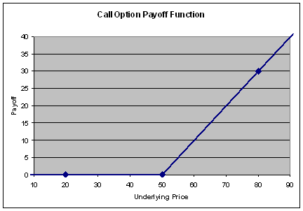
Figure 1
With these inputs, the results are as for aaOption_LV_p
above.
aaOption_LVtbl_payoff_p
Finally, we can combine the user-defined local volatility
function and the freestyle payoff by calling aaOption_LVtbl_payoff_p
with the, hopefully obvious, inputs.
Example 2: European Butterfly within
the CEV model
Today is January 1, 2007.
Consider a European butterfly option that matures 3 months from
today. It is built from two long calls
with exercise prices of $20 and $30, and two short calls with exercise prices
of $25. The current underlying price is
$25, the estimated annual volatility of the underlying is 25%, the risk-free
rate is 7.5% (annual compounding, actual/365 accrual), and the dividend rate is
2.5% (annual compounding, actual/365 accrual).
Suppose we want to value the option with the assumption
that the underlying asset undergoes a CEV evolution of the following form (the
square-root process):

with σ0
= 20% x (25)1/2 =100%. There
are various ways to do this with the FINCAD functions described above.
Since the strategy is built from European options, the
quickest, and most accurate valuation is to use the closed form solutions by
calling aaOption_LV_eu_p with the
following inputs:
aaOption_LV_eu_p
|
Argument |
Description |
Example Data |
Switch |
Comments |
|
price_u |
underlying price |
25 |
|
|
|
payoff_type |
payoff type |
13 |
butterfly |
|
|
strike_tbl |
strike table |
see below |
|
two strikes are needed to define the butterfly |
|
d_exp |
expiry date |
1-Apr-2007 |
|
3 months from today |
|
d_v |
value date |
1-Jan-2007 |
|
|
|
process |
local volatility function |
3 |
CEV |
|
|
param_tbl |
parameters for the local volatility function |
see below |
|
|
|
df_crv_std |
discount factor curve – risk free |
7.5% |
|
annual compounding and actual/365 accrual is assumed |
|
df_crv_hld |
discount factor curve – holding cost |
2.5% |
|
annual compounding and actual/365 accrual is assumed |
|
intrp |
interpolation method |
3 |
exponential |
not used for constant rates |
|
stat |
list of statistics |
1..8 |
|
|
To specify the payoff of the strategy, we need two
exercise prices (those of the long calls) in the strike_tbl:
strike_tbl
|
exercise price 1 |
exercise price 2 |
|
20 |
30 |
To specify the process, we need the two CEV
parameters in the param_tbl:
param_tbl
|
volatility |
parameter |
|
100% |
0.5 |
With these inputs, the results are:
Results
|
Output Statistics |
Description |
Value |
|
1 |
fair value |
2.988050163 |
|
2 |
delta |
-0.087035787 |
|
3 |
gamma |
-0.271404849 |
|
4 |
theta |
0.010170663 |
|
5 |
vega |
-0.083162895 |
|
6 |
rho of rate |
-0.012800295 |
|
7 |
rho of holding cost |
0.006236607 |
We can check the result using numerical
techniques by calling aaOption_LV_p with the following inputs
aaOption_LV_p
|
Argument |
Description |
Example Data |
Switch |
Comments |
|
price_u |
underlying price |
25 |
|
|
|
payoff_type |
payoff type |
13 |
butterfly |
|
|
strike_tbl |
strike table |
as above |
|
two strikes are needed to define the butterfly |
|
option_style |
option style |
1 |
European |
|
|
d_exp |
expiry date |
1-Apr-2007 |
|
3 months from today |
|
d_v |
value date |
1-Jan-2007 |
|
|
|
process |
local volatility function |
3 |
CEV |
|
|
param_tbl |
parameters for the local volatility function |
as above |
|
|
|
df_crv_std |
discount factor curve – risk free |
7.5% |
|
annual compounding and actual/365 accrual is assumed |
|
df_crv_hld |
discount factor curve – holding cost |
2.5% |
|
annual compounding and actual/365 accrual is assumed |
|
intrp |
interpolation method |
3 |
exponential |
not used for constant rates |
|
S_steps |
number of underlying steps |
200 |
|
|
|
t_steps |
number of time steps |
200 |
|
|
|
scheme |
numerical method |
1 |
Crank-Nicolson |
|
|
stat |
list of statistics |
1…8 |
|
|
With these inputs, the results are:
Results
|
Output Statistics |
Description |
Value |
|
1 |
fair value |
2.988784704 |
|
2 |
delta |
-0.086964318 |
|
3 |
gamma |
-0.271515639 |
|
4 |
theta |
0.010193946 |
|
5 |
vega |
-0.081933869 |
|
6 |
rho of rate |
-0.013154274 |
|
7 |
rho of holding cost |
0.005715143 |
|
8 |
minimum S_steps |
200 |
Since the minimum suggested number of S_steps is
200, we know that the inputs are such that we need less than 200 S_steps to
avoid any spurious numerical results.
aaOption_LV_payoff_eu_p, aaOption_LVtbl_p, aaOption_LV_payoff_p,
aaOption_LVtbl_payoff_p
The same numerical results can be obtained with a
user-defined local volatility function and/or a freestyle payoff by calling aaOption_LV_payoff_eu_p,
aaOption_LVtbl_p,
aaOption_LV_payoff_p
or aaOption_LVtbl_payoff_p. Accounting for the factors of S, the user-defined volatility to be specified in
the vol_tbl is:
 %,
giving rise to a vol_tbl which might look like:
vol_tbl
|
time |
underlying |
local volatility |
|
1-Jan-2006 |
20 |
22.36% |
|
1-Jan-2006 |
50 |
14.14% |
|
1-Jan-2006 |
80 |
11.18% |
|
1-Apr-2006 |
20 |
22.36% |
|
1-Apr-2006 |
50 |
14.14% |
|
1-Apr-2006 |
80 |
11.18% |
|
1-Jul-2006 |
20 |
22.36% |
|
1-Jul-2006 |
50 |
14.14% |
|
1-Jul-2006 |
80 |
11.18% |
although as many points as possible should be entered
in the vol_tbl for better accuracy, and the different interpolation methods
(interp_vol) should also be considered.
The payoff of the butterfly strategy is fully
specified through the following payoff_tbl:
payoff_tbl
|
underlying |
payoff |
|
15 |
0 |
|
20 |
0 |
|
25 |
5 |
|
30 |
0 |
|
45 |
0 |
which gives rise to the following piecewise linear
payoff function displayed in Figure
2:
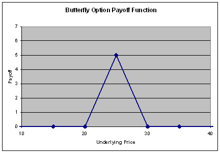
Figure 2
Example 3: Implied Volatility Skew
for the Normal Process
Today is January 1, 2007.
Suppose we have observed the implied volatilities for a range of 3 month
European options (with different exercise prices) on some underlying asset, and
have seen a distinct volatility skew.
The current underlying price is $65, the estimated annual volatility of
the return on the underlying is 15%, the risk-free rate is 7.5% (annual
compounding, actual/365 accrual), and the dividend rate is 2.5% (annual
compounding, actual/365 accrual).
Suppose we are interested in whether this volatility skew
can be reproduced by assuming that the underlying undergoes a normal process
with a volatility of 15% x 65 = 975%. To
this end, we would like to compute the implied volatilities for a range of
European options within the normal model.
We can do this by calling the FINCAD function aaOption_LV_iv with the following inputs:
aaOption_LV_iv
|
Argument |
Description |
Example Data |
Switch |
Comments |
|
price_u |
underlying price |
65 |
|
|
|
TK_tbl |
expiry dates and exercise prices |
see below |
|
maturity dates and strikes of the options for which we
want the implied volatility |
|
d_v |
value date |
1-Jan-2007 |
|
|
|
process |
local volatility function |
2 |
normal |
|
|
param_tbl |
parameters for the local volatility function |
975% |
|
the volatility of the underlying asset price |
|
df_crv_std |
discount factor curve – risk free |
7.5% |
|
annual compounding and actual/365 accrual is assumed |
|
df_crv_hld |
discount factor curve – holding cost |
2.5% |
|
annual compounding and actual/365 accrual is assumed |
|
intrp |
interpolation method |
3 |
exponential |
not used for constant rates |
The TK_tbl specifies the maturity dates and exercise
prices of the options in question. Let
us assume that this is given by:
TK_tbl
|
maturity |
exercise price |
|
1-Apr-2007 |
50 |
|
1-Apr-2007 |
55 |
|
1-Apr-2007 |
60 |
|
1-Apr-2007 |
65 |
|
1-Apr-2007 |
70 |
|
1-Apr-2007 |
75 |
|
1-Apr-2007 |
80 |
With these inputs, the results are:
Results
|
maturity |
exercise price |
implied volatility |
|
1-Apr-2007 |
50 |
17.054% |
|
1-Apr-2007 |
55 |
16.290% |
|
1-Apr-2007 |
60 |
15.611% |
|
1-Apr-2007 |
65 |
15.004% |
|
1-Apr-2007 |
70 |
14.455% |
|
1-Apr-2007 |
75 |
13.957% |
|
1-Apr-2007 |
80 |
13.502% |
We could also specify a user-defined local
volatility function and use numerical methods to generate the implied
volatilities by calling the function aaOption_LVtbl_iv. As expected, the normal model gives rise to
an implied volatility skew, which can be visualized by plotting the above
results displayed in Figure
3:
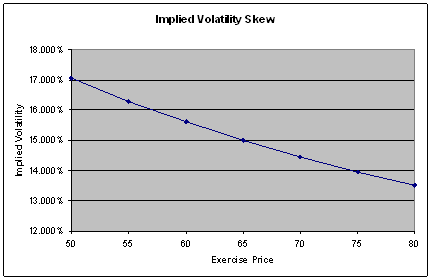
Figure 3
Related Functions
Calculates the price
and risk statistics of a standard option, a standard option strategy, or an
option portfolio, from the implied volatility smile. The function uses either closed-form
solutions or finite difference methods on the underlying no-arbitrage PDE, and
handles European and American exercise features as well as forward valuation.
Calculates the price
and risk statistics of an option with a freestyle payoff, from the implied
volatility smile. The function uses
either closed-form solutions or finite difference methods on the underlying
no-arbitrage PDE, and handles European and American exercise features as well
as forward valuation.
Calculates an
implied volatility surface and a local volatility surface, from a set of
implied volatilities. This function can
be used to expose the results of the various interpolation routines used on the
implied volatility data, and the corresponding local volatility function.
Calculates the price
and risk statistics of a European plain vanilla call or put option, a standard
European option strategy, or a user-defined portfolio of European plain vanilla
options, from the implied volatility smile.
The function interpolates implied volatilities from the smile to use in
the Black-Scholes formula.
Calculates the price
and risk statistics of a European option with a freestyle payoff, from the
implied volatility smile. The function
interpolates implied volatilities from the smile to use in the Black-Scholes
formula.
Calculates a smooth
implied volatility smile, from a set of implied volatilities. This function can be used to expose the
results of the various interpolation routines used on the implied volatility
data when pricing European options from the smile.
Calculates an
implied volatility smile, a probability distribution function (PDF) of the
underlying asset, and the skew and kurtosis of the PDF, from a set of implied
volatilities. This function can be used
to expose the results of the various interpolation routines used on the implied
volatility smile, and the resulting local volatility function, both for a single
maturity.
Calculates the fair
value and risk statistics for European style options on securities with
continuous dividend yields.
Calculates the fair
value and risk statistics for a path independent digital all-or-nothing option.
Calculates the fair
value and risk measures for an American style option where the underlying pays
a continuous dividend. Based on the Cox
Rubinstein binomial model, the function can be used for options on spot foreign
exchange or equity indexes.
Appendix A: Trading Strategies
For further details
on these strategies, and for the relevant P&L diagrams, see [11].
The call (bull) spread is a long call with exercise price  and a short call with
exercise price .
The put (bear) spread is a short put with exercise price and a long put with
exercise price .
The risk
reversal (collar) is a long put with exercise price and a short
call with exercise price  .
The seagull is a short put with exercise price , a long put with exercise price  and a short call with exercise price
 .
The straddle
is a long call and a long put, both with exercise price .
The strangle is a long put with exercise price and a long call
with exercise price .
The guts is a long call with exercise price and a long put
with exercise price .
The butterfly is a long call (or put) with exercise price , a long call (or put) with exercise price and two short
calls (or puts) with exercise price
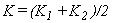 (midway between
and ). We assume
that the American butterfly consists of calls rather than puts.
The condor
is a long call (or put) with exercise
price , a long call (or put) with exercise price , a short call (or put) with exercise price  and a short
call (or put) with exercise price
 (so that the exercise
prices of the two short options are equally spaced between
 and ) . We assume
that the American condor consists of calls rather than puts.
The iron butterfly is a long straddle and a short strangle: a
short put with exercise price , a long call and a long put with exercise price and a short call with exercise price  .
The iron condor is a long strangle and a short strangle: a
short put with exercise price , a long put with exercise price , a long call
with exercise price and a short call with exercise price  .
The box
is a long call and a short put with exercise
price , and a long put and a short call with exercise price .
The ratio call spread is  short calls with exercise price and
 long calls with exercise price .
The ratio put spread is long puts with exercise price and short puts with exercise price .
The synthetic
forward is a long call and a short put, both with exercise price .
The participating
forward (put) is a long call and some percentage ( ) of a short put, both with exercise price .
The participating
forward (call) is a long put and some percentage () of a short call, both with exercise price .
The call ladder is a long call with exercise price , a short call with exercise price and a short call with exercise price  .
The put ladder is a short put with exercise price , a short put with exercise price and a long put with exercise price .
The call spread vs. put
is a long call with exercise price , a short call with exercise price and a short put with strike (usually, but not
always  ).
The put spread vs. call is a short put with exercise price , a long put with exercise price and a short call with exercise price (usually, but not always  ).
The straddle vs. call is a long call and a long put with exercise
price , and a short call with exercise price (usually, but not
always  ).
The straddle vs. put is a long call and a long put with exercise
price , and a short put with exercise price (usually, but not
always ).
References
[2]
Bachelier, L. (1900) ‘Théorie de la
spéculation’, Annales Scientifiques de l’École
Normale Supérieure, 21-86.
Reprinted in Cootner, ed. (1964) The Random
Character of Stock Market Prices,
[4]
Brigo, D. and Mercurio, F. (2000) ‘Fitting
Volatility Skews and Smiles with Analytical Stock-Price Models’, Seminar Paper
at Institute of Finance, University of Lugano.
Available on the Internet at http://www.istfin.eco.unisi.ch/seminar-papers-smile.pdf
[6]
Derman, E. and Kani,
[7]
Ding, C. G. (1992) ‘Algorithm AS275: Computing
the Non-central χ2 Distribution Function’, Applied Statistics, 41, 478-482.
[8]
Duffy, D. J. (2004), Financial
Instrument Pricing Using C++,
[9]
Dupire, B. (1994) ‘Pricing with a smile’, RISK, 7
(1), 18-20.
[10]
[11]
LIFFE Management and Administration (2002), LIFFE Options: a guide to trading strategies. Available on the Internet at http://www.euronext.com/file/view/0,4245,1626_53424_516478967,00.pdf
[12]
Merton, R. (1973) ‘Theory of Rational Option
Pricing’,
[14]
Rebonato, R. (1999) Volatility
and Correlation in the Pricing of Equity, FX and Interest-Rate Options,
[15]
Rubinstein, M. (1983) ‘Displaced Diffusion
Option Pricing’, Journal of Finance, 38, 213-217.
[16]
Wilmott, P. (2006) Paul
Wilmott on Quantitative Finance, 2nd ed.,
Disclaimer
With respect to this document,
FinancialCAD Corporation (“FINCAD”) makes no warranty either express or
implied, including, but not limited to, any implied warranty of merchantability
or fitness for a particular purpose. In no event shall FINCAD be liable to
anyone for special, collateral, incidental, or consequential damages in
connection with or arising out of the use of this document or the information
contained in it. This document should not be relied on as a substitute for your
own independent research or the advice of your professional financial,
accounting or other advisors.
This information is subject to change
without notice. FINCAD assumes no responsibility for any errors in this
document or their consequences and reserves the right to make changes to this
document without notice.
Copyright
Copyright ©
FinancialCAD Corporation 2008. All rights reserved.


